(paper 85) SSL for TS Analysis; Taxonomy, Progress, and Prospects

SSL for TS Analysis: Taxonomy, Progress, and Prospects

Contents

1. Abstract
2. Introduction

0. Abstract

Reduces the dependence on labeled data.

Review current SOTA SSL methods for TS

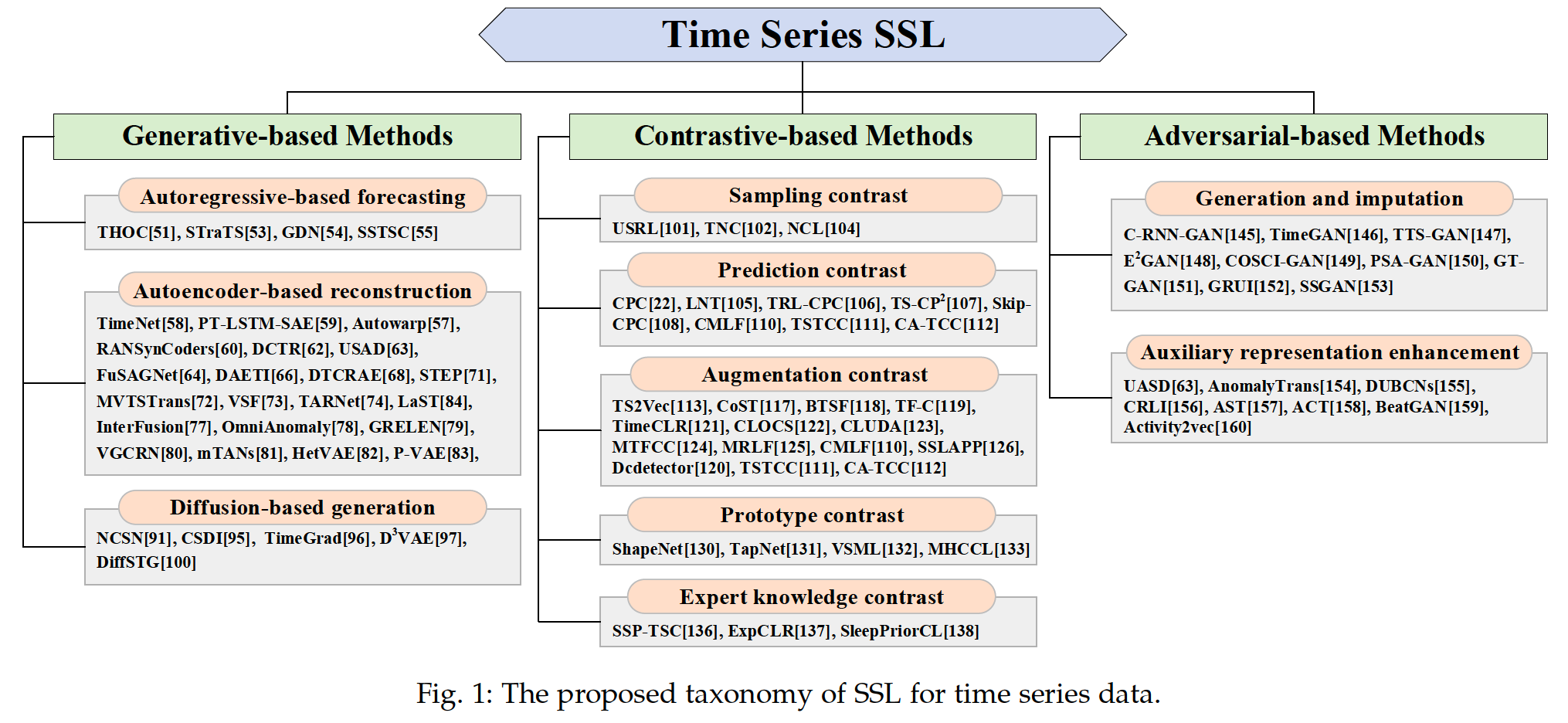
Provide a new taxonomy of existing TS SSL methods

• (1) Generative-based
• (2) Contrastive-based
• (3) Adversarial-based

( All methods can be further divided into 10 subcategories )

Tasks : TS forecasting, classification, anomaly detection, and clustering tasks

1. Introduction

Transferring the pretext tasks designed for CV/NLP directly to TS

\(\rightarrow\) often fails to work in many scenarios.

Challenges :

(1) TS exhibit unique properties

• ex) seasonality, trend, and frequency domain information
• pretext tasks designed for CV/NLP : do not consider these semantics

(2) Data augmentation need to be specially designed for TS

• ex) rotation and crop : may break the temporal dependency of TS

(3) TS data contain multiple dimensions ( = MTS )

• useful information usually only exists in a few dimensions,

  making it difficult to extract useful information in TS using SSL methods for other data types.

Three perspectives:

• (1) generative-based
• (2) contrastive-based
• (3) adversarial-based.

a) Generative-based

Three frameworks:

• (1) autoregressive-based forecasting
• (2) auto-encoder-based reconstruction
• (3) diffusion-based generation.

b) Contrastive-based

Five categories based on how positive and negative samples are generated

• (1) sampling contrast
• (2) prediction contrast
• (3) augmentation contrast
• (4) prototype contrast
• (5) expert knowledge contrast.

For each category, we analyze its insights and limitations.

c) Adversarial-based

Based on two target tasks:

• (1) time series generation/imputation
• (2) auxiliary representation enhancement

Section 2

• provides some review literature on SSL and TS data

Section 3 ~ 5

• describe the generation-based, contrastive-based, and adversarial-based methods

Section 6

• commonly used TS datasets from the application perspective

Section 7

• several promising directions of TS SSL

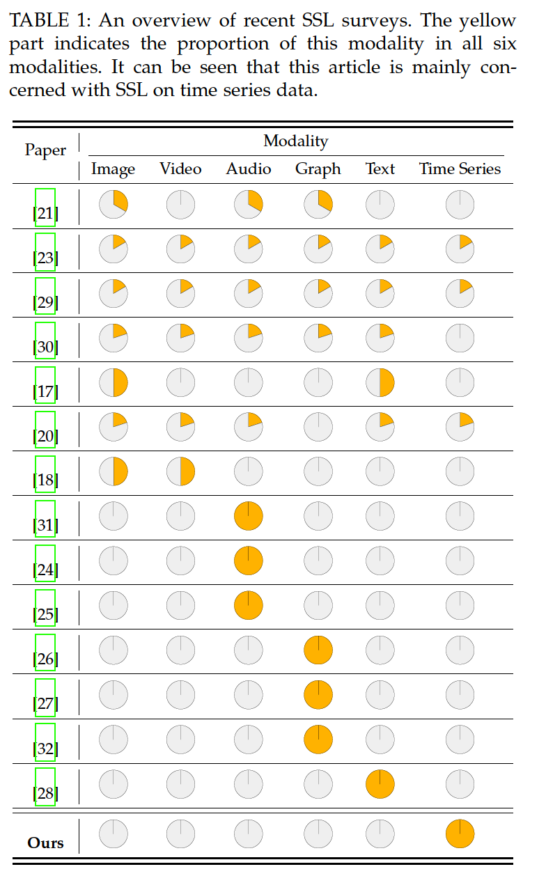
2. Related Surveys

4 widely used criteria

• (1) Learning paradigms
• (2) Pretext tasks
• (3) Components/modules
• (4) Downstream tasks

(1) Surveys on SSL

a) Learning paradigms

Model architectures & Training objectives.

• (1) generative-based
• (2) contrastive-based
• (3) adversarial-based methods

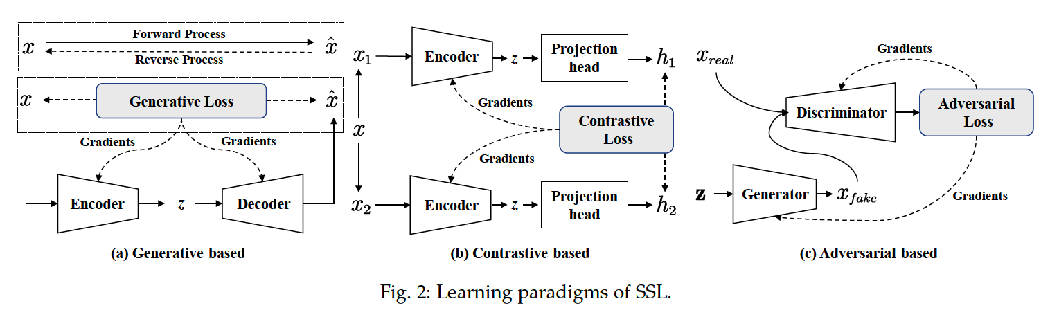
Generative-based approach

• Encoder : \(\mathbf{x} \rightarrow \mathbf{z}\)
• Training objective : Reconstruction error

Contrastive-based approach

• most widely used SSL strategies
• constructs positive and negative samples via data augmentation or context sampling
• trained by maximizing the Mutual Information (MI) between the two positive samples.
  • ex) InfoNCE loss

Adversarial-based approach

• consists of a generator and a discriminator.

b) Pretext Tasks

Five broad families:

• (1) transformation prediction
• (2) masked prediction
• (3) instance discrimination
• (4) clustering
• (5) contrastive instance discrimination.

c) Components and modules

Four components:

• (1) positive and negative samples
• (2) pretext task
• (3) model architecture
• (4) training loss.

Step 1) construct true positive and negative samples

• choice of data augmentation techniques depends on the data modality
• ex) image
  • crop, color distort, resize, and rotate
• ex) TS
  • noise injection, window slicing, and window wrapping

Step 2) pretext tasks

Step 3) model architecture

• determines how positive and negative samples are encoded during training.
• ex) end-to-end, memory bank, momentum encoder, and clustering

d) Downstream tasks

pass

(2) Surveys on TS data

Two categories

Category 1) Tasks

• classification, forecasting, anomaly detection

Category 2 ) Key components of TS modeling

• data augmentation, model structure

3. Generative-based Methods

TS modeling

• using the past series to forecast the future windows
• using the encoder and decoder to reconstruct the input
• forecasting the unseen part of the masked time series.

Categories

• Autoregressive-based forecasting

• Autoencoder-based reconstruction

• Diffusion-based generation

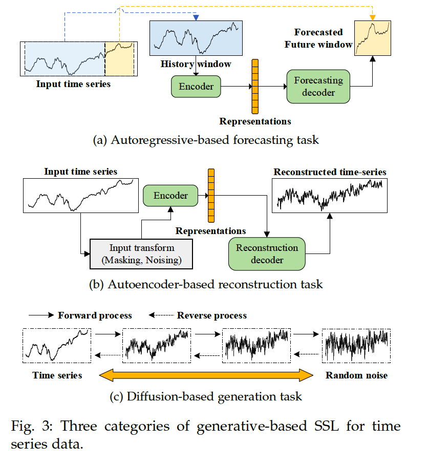
(1) Autoregressive-based forecasting (ARF)

Goal : \(\hat{X}_{[t+1: t+K]}=f\left(X_{[1: t]}\right)\).

Learning objective : \(\mathcal{L}=D\left(\hat{X}_{[t+1: t+K]}, X_{[t+1: t+K]}\right)\).

• usually MSE : \(\mathcal{L}=\frac{1}{K} \sum_{k=1}^K\left(\hat{X}_{[t+k]}-X_{[t+k]}\right)^2\)

ARF as a pretext task

• RNNs
  • ex) THOC : constructs a SSL pretext task for multi-resolution single-step forecasting called Temporal Self-Supervision (TSS).
    • structure : L-layer dilated RNN with Skip-Connection
• CNNs
  • ex) STraTS :
    • encodes the TS into triple representations to avoid the limitations of using basic RNN and CNN in modeling irregular and sparse time series data
    • builds the transformer-based forecasting model for modeling medical MTS
• Graph-based
  • GNNs can better capture the correlation between variables in MTS (ex. GDN)

SSTSC

• proposes a temporal relation learning prediction task based on the “PastAnchor-Future” strategy as SSL pretext task
  • forecasting the values of the future time windows (X)
  • predicts the relationships of the time windows (O)

(2) Autoencoder-based reconstruction

AE : \(Z=E(X), \quad \tilde{X}=D(Z)\).

Goal : \(\mathcal{L}=\|X-\tilde{X}\|_2\)

TimeNet, PT-LSTM-SAE, Autowarp

• use RNN AE

Zhang et al. [61]

• use CNN-based AE

Abdulaal et al. [60]

• focus on the complex asynchronous MTS
• introduce the spectral analysis in the AE
• synchronous representation of the TS?
  • extracted by learning the phase information in the data
  • used for the anomaly detection task

DTCR [62]

• temporal clustering-friendly representation learning model.
• k-means constraints in reconstruction

USAD [63]

• 1 encoder & 2 decoders
• introduce adversarial training

FuSAGNet [64]

• introduces graph learning on sparse AE to model relationships btw MTS

Denoisining AE

• \(X_n=\mathcal{T}(X), \quad Z=E\left(X_n\right), \quad \tilde{X}=D(Z)\),
• noise example
  • adding Gaussian noise
  • randomly setting some time steps to zero

Mask autoencoder (MAE)

• \(X_m=\mathcal{M}(X), \quad Z=E\left(X_m\right), \quad \tilde{X}=D(Z)\),

• objective function
  • \(\mathcal{L}=\mathcal{M}\left(\|X-\tilde{X}\|_2\right)\).
  • loss of MAE is only computed on the masked part.
• Masking in TS
  • time-step-wise masking
    • Good ) finegrained info
    • Bad) contextual semantic info
  • segment-wise masking
    • pay more attention to slow features in the TS
    • ex) trends or high-level semantic info
  • variable-wise masking

STEP [71]

• MAE ( segment-wise masking )

• divided the series into multiple non-overlapping segments ( of equal length )

  randomly selected a certain proportion of the segments for masking.

• 2 advantages of using segment-wise masking

  • (1) capture semantic information
  • (2) computational efficiency : reduce the input length to the encoder

TST ( Zerveas et al. [72] )

• performed a more complex masking operation on TS
• MTS was randomly divided into multiple non-overlapping segments of unequal length on each variable.

Chauhan et al. [73]

• introduce variable-wise masking
• define new TS forecasting task : Variable Subset Forecast (VSF)
  • TS for trraining & inference : different dimensions or variables
    • due to absence of some sensor data.
  • feasibility of SSL based on variable-wise masking

TARNet [74]

• propose new masking strategy
  • random masking (X)
  • data-driven masking strategy (O)
    • uses self-attention score distribution from downstream task
    • masks out these necessary time steps

Variational autoencoder (VAE)

• \(P(Z \mid X)=E(X), \quad Z=\mathcal{S}(P(Z \mid X)), \quad \tilde{X}=D(Z)\).
  • \(\mathcal{S}(\cdot)\) : sampling operation
• Loss term : \(\mathcal{L}=\|X-\tilde{X}\|_2+\operatorname{KL}(\mathcal{N}(\mu, \delta), \mathcal{N}(0, I))\)
  • reconstruction item & regularization item
• ex) InterFusion [77]
  • hierarchical VAE
  • models inter-variable and temporal dependencies
• ex) OmniAnomaly [78]
  • Interpretable TS AD algorithm
  • combines VAE and Planar Normalizing Flow
• ex) GRELEN [79] and VGCRN [80]
  • introduce the graph structure and in VAE.

Methods based on VAE

• have made progress in sparse and irregular TS
  • ex) mTANs [81], HetVAE [82] and P-VAE [83].
• recent works
  • extract seasonal and trend representations in TS based on VAE
  • ex) LaST [84]
    • disentangled VI framework with MI constraints
    • separates seasonal and trend representations in the latent space

(3) Diffusion-based generation

Key design of the diffusion model: 2 inverse processes:

• (1) Forward process
  • injecting random noise
• (2) Reverse process
  • sample generation from noise distribution

Three basic formulations of diffusion models

• (1) Denoising diffusion probabilistic models (DDPMs)
• (2) Score matching diffusion models
• (3) Score SDEs

a) DDPMs

Two Markov chains

• (1) Forward chain
  • adds random noise to data
• (2) Reverse chain
  • transforms noise back into data.

Data distribution : \(\boldsymbol{x}_0 \sim q\left(\boldsymbol{x}_0\right)\)

Forward Markov process :

• transition kernel \(q\left(\boldsymbol{x}_t \mid \boldsymbol{x}_{t-1}\right)\).
  • usually set as \(q\left(\boldsymbol{x}_t \mid \boldsymbol{x}_{t-1}\right)=\mathcal{N}\left(\boldsymbol{x}_t ; \sqrt{1-\beta_t} \boldsymbol{x}_{t-1}, \beta_t I\right)\)
• joint pdf \(\boldsymbol{x}_1, \boldsymbol{x}_2, \ldots, \boldsymbol{x}_T\) conditioned on \(\boldsymbol{x}_0\) :
  • \(q\left(\boldsymbol{x}_1, \boldsymbol{x}_2, \ldots, \boldsymbol{x}_T \mid \boldsymbol{x}_0\right)=\prod_{t=1}^T q\left(\boldsymbol{x}_t \mid \boldsymbol{x}_{t-1}\right)\).

Backward Markov process

• \(p\left(\boldsymbol{x}_T\right)=\mathcal{N}\left(\boldsymbol{x}_T ; 0, I\right)\).
• joint pdf : \(p_\theta\left(\boldsymbol{x}_0, \boldsymbol{x}_1, \ldots, \boldsymbol{x}_T\right)=p\left(\boldsymbol{x}_T\right) \prod_{t=1}^T p_\theta\left(x_{t-1} \mid x_t\right)\),
  • \(p_\theta\left(\boldsymbol{x}_{\boldsymbol{t}-\mathbf{1}} \mid \boldsymbol{x}_{\boldsymbol{t}}\right)=\) \(\mathcal{N}\left(\boldsymbol{x}_{t-1} ; \mu_\theta\left(\boldsymbol{x}_t, t\right), \sum_\theta\left(\boldsymbol{x}_t, t\right)\right)\).

Goal : minimize KL-div btw 2 joint distns

• \(\begin{array}{r} \mathbf{K L}\left(q\left(\boldsymbol{x}_1, \boldsymbol{x}_2, \ldots, \boldsymbol{x}_T\right) \| p_\theta\left(\boldsymbol{x}_0, \boldsymbol{x}_1, \ldots, \boldsymbol{x}_T\right)\right) \geq \mathbf{E}\left[-\log p_\theta\left(\boldsymbol{x}_0\right)\right]+\text { const } \end{array}\).

b) Score matching diffusion models

Notation :

• pdf : \(p(\boldsymbol{x})\)
• Stein score : \(\nabla_x \log p(\boldsymbol{x})\)
  • gradient of the log density function of the input data \(\boldsymbol{x}\),
  • points to the directions with the largest growth rate in pdf

Key idea :

• perturb data with a sequence of Gaussian noise
• then jointly estimate the score functions for all noisy data distributions by training a DNN conditioned on noise levels.
• Why? Much easier to model and estimate the score function than the original pdf

Langevin dynamics

• ( step size \(\alpha>0\), a number of iterations \(T\) , initial sample \(x_0\) )

• iteratively does the following estimation to gain a close approximation of \(p(\boldsymbol{x})\)

  \(\boldsymbol{x}_t \leftarrow \boldsymbol{x}_{t-1}+\alpha \nabla_x \log p\left(\boldsymbol{x}_{t-1}\right)+\sqrt{2 \alpha} \boldsymbol{z}_t, 1 \leq t \leq T\).

  • where \(z_t \sim \mathcal{N}(0, I)\).

• However, the score function is inaccurate without the training data, and Langevin dynamics may not converge correctly.

NCSN (a noise-conditional score network)

• perturbing data with a noise sequence
• jointly estimating the score function for all the noisy data conditioned on noise levels

c) Score SDEs

DDPMs & SGMs

• limited to discrete and finite time steps

Score SDEs

• process the diffusion operation according to the stochastic differential equation
• \(d \boldsymbol{x}=f(\boldsymbol{x}, t) d t+g(t) d \boldsymbol{w}\),
  • where \(f(\boldsymbol{x}, t)\) and \(g(t)\) are diffusion function and drift function of the SDE
  • \(\boldsymbol{w}\) : standard Wiener process.

Score SDEs generalize the diffusion process to the case of infinite time steps

Fortunately, DDPMs and SGMs also can be formulated with corresponding SDEs.

• DDPMs : \(d \boldsymbol{x}=-\frac{1}{2} \beta(t) \boldsymbol{x} d t+\sqrt{\beta(t)} d \boldsymbol{w}\)
  • where \(\beta\left(\frac{t}{T}\right)=T \beta_t\) when \(\mathrm{T}\) goes to infinity
• SGMs : \(d \boldsymbol{x}=\sqrt{\frac{d\left[\delta(t)^2\right]}{d t}} d \boldsymbol{w}\)
  • where \(\delta\left(\frac{t}{T}\right)=\delta_t\) as \(\mathrm{T}\) goes to infinity.

With any diffusion process in the form of \(d \boldsymbol{x}=f(\boldsymbol{x}, t) d t+g(t) d \boldsymbol{w}\),

\(\rightarrow\) reverse process can be gained by ..

• \(d \boldsymbol{x}=\left[f(\boldsymbol{x}, t)-g(t)^2 \nabla_{\boldsymbol{x}} \log q_t(\boldsymbol{x})\right] d t+g(t) d \overline{\boldsymbol{w}}\).
  • \(\overline{\boldsymbol{w}}\) : a standard Wiener process when time flows reversely
  • \(d t\) :an infinitesimal time step.

Besides that, the existence of an ordinary differential equation, which is also called the probability flow \(O D E\), is defined as follows. \(d \boldsymbol{x}=\left[f(\boldsymbol{x}, t)-\frac{1}{2} g(t)^2 \nabla_{\boldsymbol{x}} \log q_t(\boldsymbol{x})\right] d t .\) The trajectories of the probability flow ODE have the same marginals as the reverse-time SDE. Once the score function at each time step is known, the reverse SDE can be solved with various numerical techniques. Similar objective is designed with SGMs.

Diffusion models have also been applied in time series analysis recently. We will briefly introduce some of them, including the designed architectures and the main diffusion techniques used. 3.3.4 Diffusion models for time series imputation Conditional Score-based Diffusion Models for Imputation (CSDI) [95] proposes a novel time series imputation method that utilizes score-based diffusion models conditioned on observed data. It is trained for imputation and can be easily