(paper 95) CALDA; Improving Multi-Source Time Series Domain Adaptation with Contrastive Adversarial Learning

CALDA: Improving Multi-Source Time Series Domain Adaptation with Contrastive Adversarial Learning

https://arxiv.org/pdf/2109.14778.pdf

Contents

1. Abstract
2. Introduction

0. Abstract

Unsupervised domain adaptation (UDA)

CALDA : combines CL & AL to support MS-UDA for TS data

• CL : Contrastive Learning
  • pull/push same/different labels
• AL : Adversarial Learning
  • to align source and target
• MS-UDA : Multi-Source UDA
• Details
  • Leverages cross-source label information across domains
  • Requires neither data augmentation nor pseudo labeling

Experiments

• utilizing cross-source information improves performance over prior time series and contrastive methods.
• Weak supervision further improves performance, even in the presence of noise

1. Introduction

Multi-Source Unsupervised Domain Adaptation (MSUDA)

• train based on labeled data from the source
• when performing adaptation, must bridge a domain gap

Model for time-series MS-UDA. uses …

• labeled data : from one or more source domains
• unlabeled data : from a target domain
• optional target class distribution.

Existing approaches to adaptation do not make effective use of meta-domain information about the target

\(\rightarrow\) additional gains may stem from leveraging this information via weak supervision

CALDA

(Contrastive Adversarial Learning for Multi-Source Time Series Domain Adaptation)

• improves UDA via AL & CL & Weak-supervision
• does not use DA or pseudo-labeling

[1] AL ( Multi-source domain AL )

trains a multiclass domain classifier

• encoder : to incorrectly predict the example’s domain.

• result : domain-invariant features

  ( = align the feature-level distributions between domains )

[2] CL

to leverage cross-source label information

( for improving accuracy on the target domain )

• widely used in SSL, but unexplored for multi-source TS DA

3 design decisions

• (Design 1) select pairs of examples from source domains
• (Design 2) determine whether it is beneficial to pseudo-label and include target data as a contrastive learning domain despite the likelihood of incorrect pseudo-labels due to the large domain shifts in time series data.
• (Design 3) randomly select? select hard examples?

Design 1)

• hypothesize that cross-source information to select example pairs can improve transfer

Design 2)

• perform CL only on source ( not on pseudo-labeled target )
• Why NOT?
  • (a) due to risk of being incorrectly labeled
  • (b) since CALDA employs more than one source domain, can perform CL between source domains

Design 3)

• hard examples do not need to be singled out

  ( such examples already intrinsically yield a greater contribution to the CL )

• hypothesize that both random and hard sampling may offer improvements for multi-source domain adaptation

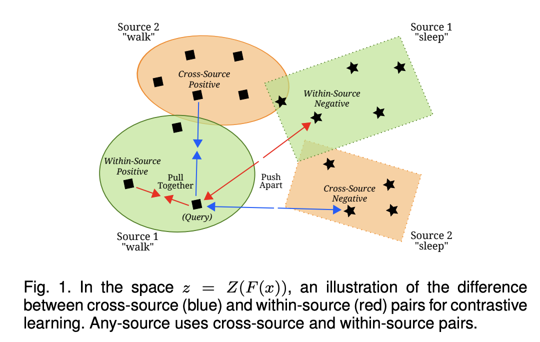
( Design 1 figure )

Contributions

• (1) Improve upon existing time-series MS-UDA by leveraging cross-source domain labels via CL, without requiring data augmentation or pseudo labeling.
• (2) Incorporate multiple CL strategies into CALDA to analyze the impact of design choices.
• (3) Offer an approach to time series MS-UDA that makes use of class distribution information where available through weak supervision.

2. Related Work

(1) DA

Multi-source DA

• Zhao et al. [15] : adversarial method supporting multiple sources by including a binary domain classifier for each source
• Ren et al. [16] : align the sources, merging them into one domain that is aligned to the target
• Li et al. [17] : also unify multiple source domains

\(\rightarrow\) these approaches, however, do not take advantage of example similarities through CL to effectively use source labels

Xie et al. [18]

• propose a scalable method, only requiring one multi-class domain classifier

  ( similar to AL in CALDA )

Yadav et al.

• use CL when combining multiple sources.

• CL achieves higher intraclass compactness across domains

  \(\rightarrow\) yielding well-separated decision boundaries

( Architecture )

• for both single- & multi-source DA, 1D-CNN > RNN
• thus use 1D-CNN in CALDA

(2) CL

pass

3. Problem Setup

Formalize MS-UDA (Multi-Source UDA) w/ & w/o weak supervision

(1) MS-UDA

Assumption

• (1) labeled data : from multiple sources
• (2) unlabeled data : from the target source

Goal : model that performs well on the target domain

Data distribution

• Source distributions : \(\mathcal{D}_{S_i}\) for \(i \in\{1,2, \ldots, n\}\)
• Target distribution : \(\mathcal{D}_T\)

Procedure

• draw \(s_i\) labeled training examples from each source distn \(\mathcal{D}_{S_i}\)
• draw \(t_{\text {train }}\) unlabeled training instances from marginal distn \(\mathcal{D}_T^X\)

\(\begin{gathered} S_i=\left\{\left(\mathbf{x}_j, y_j\right)\right\}_{j=1}^{s_i} \sim \mathcal{D}_{S_i} \quad \forall i \in\{1,2, \ldots, n\} \\ T_{\text {train }}=\left\{\left(\mathbf{x}_j\right)\right\}_{j=1}^{t_{\text {train }}} \sim \mathcal{D}_T^X \end{gathered}\).

Each domain is distributed over the space \(X \times Y\),

• \(X\) : input data space
• \(Y\) : label space \(Y=\{1,2, \ldots, L\}\) for \(L\) classification labels.

MS-UDA model \(f: X \rightarrow Y\)

• train the model using \(S_i\) and \(T_{\text {train }}\)
• test the model using a holdout set of \(t_{\text {test }}\) labeled testing examples from \(\mathcal{D}_T\)
  • \(T_{\text {test }}=\left\{\left(\mathbf{x}_j, y_j\right)\right\}_{j=1}^{t_{\text {test }}} \sim \mathcal{D}_T\).

Time series data

\(X=\) \(\left[X^1, X^2, \ldots, X^K\right]\) for \(K\) channels

• each variable \(X^i=\left[x_1, x_2, \ldots, x_H\right]\) ( \(H\) time steps )

(2) MS-UDA with Weak Supervison

Target-domain label proportions are additionally available during training

• represent \(P(Y=y)\) for the target domain
  • \(Y_{\text {true }}(y)=P(Y=y)=p_y\).
  • probability \(p_y\) that each example will have label \(y \in\{1,2, \ldots, L\}\)

4. CALDA Framework

MS-UDA framework that blends (1) AL & (2) CL

1. Motivate CALDA from domain adaptation theory.

2. Key components:
   1. source domain error minimization
   2. AL
   3. CL
3. Framework alternatives to investigate how to best construct the example sets used in contrastive loss.

(1) Theoretical Motivation

Zhao et al. [15] offer an error bound for multi-source domain adaptation.

Notation

• Hypothesis space \(\mathcal{H}\) with VC-dimension \(v\)
• \(n\) source domains
• Empirical risk \(\hat{\epsilon}_{S_i}(h)\) of the hypothesis on source domain \(S_i\) for \(i \in\{1,2, \ldots, n\}\)
• Empirical source distributions \(\hat{\mathcal{D}}_{S_i}\) for \(i \in\{1,2, \ldots, n\}\)
  • generated by \(m\) labeled samples from each source domain
• Empirical target distribution \(\hat{\mathcal{D}}_T\)
  • generated by \(m n\) unlabeled samples from target domain
• Optimal joint hypothesis error \(\lambda_\alpha\) on a mixture of source domains \(\sum_{i \in[n]} \alpha_i S_i\)
• Target domain \(T\) (average case if \(\alpha_i=1 / n \forall i \in\{1,2, \ldots n\}\) )
• Target classification error bound \(\epsilon_T(h)\) with probability at least \(1-\delta\) for all \(h \in \mathcal{H}\)

\(\begin{aligned} \epsilon_T(h) & \leq \sum_{i=1}^n \alpha_i(\overbrace{\hat{\epsilon}_{S_i}(h)}^{(1) \text { source errors }}+\underbrace{\frac{1}{2} d_{\mathcal{H} \Delta \mathcal{H}}\left(\hat{\mathcal{D}}_T ; \hat{\mathcal{D}}_{S_i}\right)}_{\text {(2) divergences }}) \\ & +\overbrace{\lambda_\alpha}^{\text {(3) opt. joint hyp. }}+\underbrace{O\left(\sqrt{\frac{1}{n m}\left(\log \frac{1}{\delta}+v \log \frac{n m}{v}\right)}\right)}_{\text {(4) due to finite samples }} \end{aligned}\).

Term (1) = sum of source domain errors

Term (2) = sum of the divergences between each source domain and the target

Term (3) = optimal joint hypothesis on the mixture of source domains and the target domain,

Term (4) = due to finite sample sizes

\(\rightarrow\) Term (1) & (2) are the most relevant for informing multi-source domain adaptation methods since they can be optimized.

Introduce CALDA to minimize this error bound!

Step 1) train a Task Classifier

( = minimizing (1) )

Step 2) better align domains based on AL & CL

( = minimizing (2) )

• (As in prior works) domain adversarial training

  • to align the sources and unlabeled data from the target domain.

• (NEW) propose a supervised contrastive loss

  • to align the representations of same-label examples among the multiple source domains

    \(\rightarrow\) helps determining which aspects of the data correspond to differences in the class label (the primary concern) versus differences in the domain where the data originiated

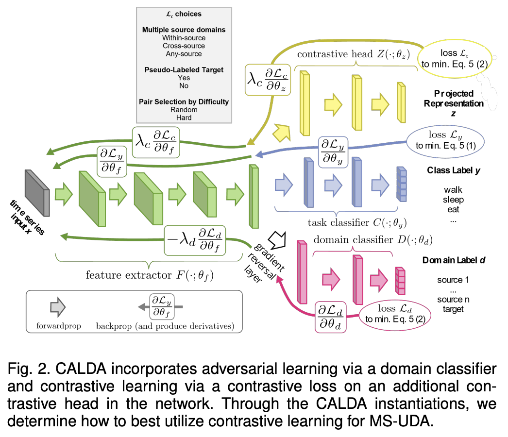
(2) Adaptation Components

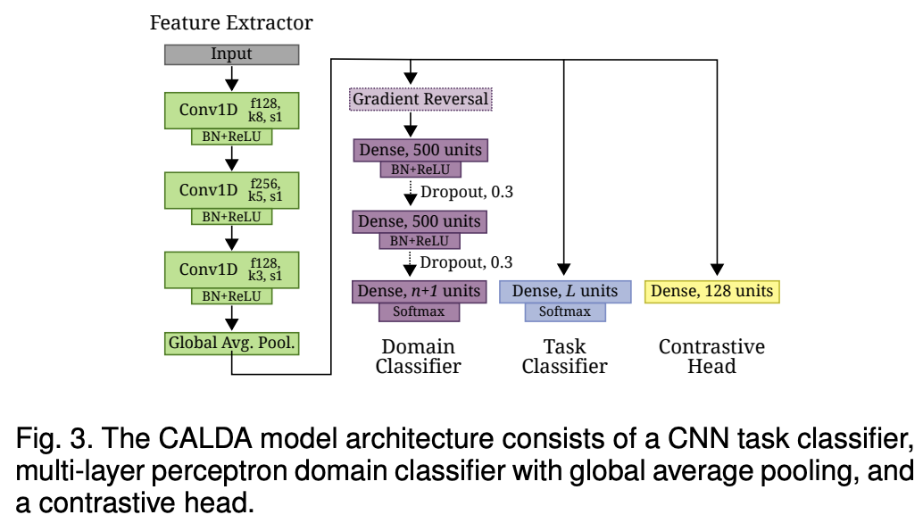
Architecture

• \(F\left(\cdot ; \theta_f\right)\): feature extractor (1D-CNN layers … with GAP for variable length)
• \(C\left(\cdot ; \theta_c\right)\): task classifier (Dense layer)
• \(D\left(\cdot ; \theta_d\right)\) : domain classifier (MLP)
• contrastive head

a) Source Domain Errors

\(\underset{\theta_f, \theta_c}{\arg \min } \sum_{i=1}^n \underset{(x, y) \sim \mathcal{D}_{S_i}}{\mathbb{E}}\left[\mathcal{L}_y(y, C(F(x)))\right]\).

• for source domain datasets
• CE loss

b) Adversarial Learning

( Key : gradient reversal layer \(\mathcal{R}(\cdot)\) between \(F\) and \(D\) )

\(\begin{aligned} \underset{\theta_f, \theta_d}{\arg \min } & \sum_{i=1}^n \underset{(x, y) \sim \mathcal{D}_{S_i}}{\mathbb{E}}\left[\mathcal{L}_d\left(d_{S_i}, D(\mathcal{R}(F(x)))\right)\right] \\ & +\underset{x \sim \mathcal{D}_T^X}{\mathbb{E}}\left[\mathcal{L}_d\left(d_T, D(\mathcal{R}(F(x)))\right)\right] \end{aligned}\).

c) Contrastive Learning

Supervised contrastive loss ( based on a multiple-posiftive InfoNCE loss )

• \(\begin{aligned} & \mathcal{L}_c(z, P, N)= \\ & \frac{1}{ \mid P \mid } \sum_{z_p \in P}\left[-\log \left(\frac{\exp \left(\frac{\operatorname{sim}\left(z, z_p\right)}{\tau}\right)}{\sum_{z_k \in N \cup\left\{z_p\right\}} \exp \left(\frac{\operatorname{sim}\left(z, z_k\right)}{\tau}\right)}\right)\right] \end{aligned}\).
  • \(P\) : positive sets
  • \(N\) :negative sets

( If pseudo-labeled version : )

\(\begin{aligned} & \underset{\theta_f, \theta_z}{\arg \min } \sum_{i=1}^n\left[\frac{1}{ \mid Q_{S_i} \mid } \sum_{\left(z_q, y_q\right) \in Q_{S_i}} \mathcal{L}_c\left(z_q, P_{d_{S_i}, y_q}, N_{d_{S_i}, y_q}\right)\right] \\ & +\mathbf{1}_{P L=\text { True }} \frac{1}{ \mid Q_T \mid } \sum_{\left(z_q, \hat{y}_q\right) \in Q_T} \mathcal{L}_c\left(z_q, P_{d_T, \hat{y}_q}, N_{d_T, \hat{y}_q}\right) \end{aligned}\).

d) Total Loss & Weak Supervision Regularizer

Jointly train each of these three adaptation components

Total loss = sum of 3 losses

• (1) source domain errors
• (2) adversarial learning
  • \(\lambda_d\) multiplier included in \(\mathcal{R}(\cdot)\) can be used as a weighting parameter for the adversarial loss.
• (3) contrastive learning
  • further add a weighting parameter \(\lambda_c\) for CL loss

MS-UDA with weak supervision

• weak supervision settings
  • individual labels for the unlabeled target domain data are unknown
  • but distribution is known
• include the (4) weak supervision regularization term
• \(\underset{\theta_f, \theta_c}{\arg \min }\left[D_{K L}\left(Y_{\text {true }} \mid \mid \mathbb{E}_{x \sim \mathcal{D}_T^X}[C(F(x))]\right)\right]\).
• KL-divergence regularization term guides the training

(3) Design Decisions for Contrastive Learning

Questions

• Q1) how to select example pairs across multiple domains
• Q2) whether to include a pseudo-labeled target domain in CL
• Q3) whether to select examples randomly or based on difficulty.

a) Multiple Source Domains

May choose to select two examples ..

• (1) Within-Source : from a single domain
• (2) Cross-Source : from two different domains
• (3) Any-Source : combination.

Distinguished based on whether \(d=d_q\) (Within-Source), \(d \neq d_q\) (Cross-Source), or there is no constraint (Any-Source).

(1) Within-Source Label-CL

\(\begin{aligned} & P_{d_q, y_q}=\left\{z \mid(x, y, d) \in K, z=Z(F(x)), d=d_q, y=y_q\right\} \\ & N_{d_q, y_q}=\left\{z \mid(x, y, d) \in K, z=Z(F(x)), d=d_q, y \neq y_q\right\} \end{aligned}\).

(2) Any-Source Label-CL

\(\begin{aligned} & P_{d_q, y_q}=\left\{z \mid(x, y, d) \in K, z=Z(F(x)), y=y_q\right\} \\ & N_{d_q, y_q}=\left\{z \mid(x, y, d) \in K, z=Z(F(x)), y \neq y_q\right\} \end{aligned}\).

(3) Cross-Source Label-CL

\(\begin{aligned} & P_{d_q, y_q}=\left\{z \mid(x, y, d) \in K, z=Z(F(x)), d \neq d_q, y=y_q\right\} \\ & N_{d_q, y_q}=\left\{z \mid(x, y, d) \in K, z=Z(F(x)), d \neq d_q, y \neq y_q\right\} \end{aligned}\).

b) Pseudo-Labeled Target Domain

TL= True > TL = False

c) Pair Selection by Difficulty

Model prediction \(\hat{y}=\arg \max C(F(x))\)

option 1) Define hard positive and negative sets \(\bar{P}\) and \(\bar{N}\)

\(\begin{gathered} \bar{P}_{d_q, y_q}=\{z \mid(x, y, d) \in K, z=Z(F(x)) \\ \left.d \neq d_q, y=y_q, \hat{y} \neq y_q\right\} \\ \bar{N}_{d_q, y_q}=\{z \mid(x, y, d) \in K, z=Z(F(x)) \\ \left.d \neq d_q, y \neq y_q, \hat{y}=y_q\right\} \end{gathered}\).

option 2) Define relaxed hard positive and negative sets \(\tilde{P}\) and \(\tilde{N}\)

\(\begin{gathered} \tilde{P}_{d_q, y_q}=\left\{z \mid(x, y, d) \in K, z=Z(F(x)), d \neq d_q, y=y_q\right. \\ \left.\mathcal{L}_y(y, C(F(x)))>h_p\right\} \\ \tilde{N}_{d_q, y_q}=\left\{z \mid(x, y, d) \in K, z=Z(F(x)), d \neq d_q, y \neq y_q\right. \\ \left.\mathcal{L}_y\left(y_q, C(F(x))\right)<h_n\right\} \end{gathered}\).