DiffLoad; Uncertainty Quantification in Electrical Load Forecasting with the Diffusion Model

DiffLoad: Uncertainty Quantification in Electrical Load Forecasting with the Diffusion Model

Contents

1. Abstract
2. Introduction
3. Proposed Methods
   1. Epistemic uncertainty
   2. Aleatoric uncertainty
   3. Two kinds of uncertainties

0. Abstract

Uncertainties in loadd forecasting

• (1) Epistemic ( = model ) uncertainty
• (2) Aleatoric ( = data ) uncertainty

This paper proposes ..

• (1) Diffusion-based Seq2Seq to estimate “epistemic” uncertainty
• (2) Additive Cauchy distribution to estimate “aleatoric” uncertainty

1. Introduction

Previous diffusion TS methods ( i.e. TimeGrad )

• Provide probabilistic forecasts to capture uncertainties

• But do not clearly define what uncertainty they were modeling

Drawbacks of previous DL methods to capture uncertainties

• (1) Bayesian NN / Ensemble …
  • Very expensive
    • Bayesian NN: treats NN parammeters as r.v.
    • Ensemble: requires multiple models
  • Relies on Gaussian distn … limit the model’s expressive power & easily affected by noise
• (2) Dropout
  • Pros) Do not require assumptions
  • Cons) Foreacasting perormance is unstable due to inconsistencies in training & testing

Proposed

Develop a new uncertainty quantification framework

• Estimate and separate 2 kinds of uncertainties
• (1) Aleatoric (data) uncertainty
  • apply a heavy-tailed emission head
  • reduce the bad efffect caused by noise
• (2) Epistmeic (model) uncertainty
  • propose a diffusion-based framework to concentrate on the uncertainty of the model on the hidden state
  • do not increase computational burden much!

2. Proposed Methods

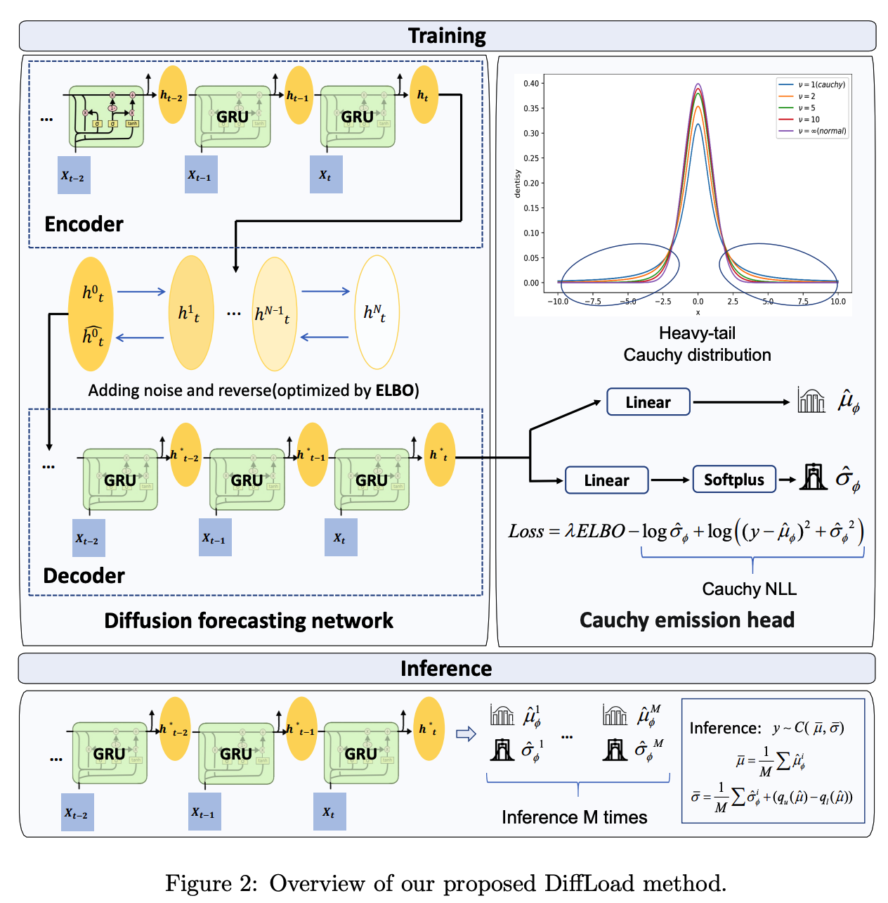
1. Diffusion Forecasting network
   • based on Seq2Seq
   • for epistemic uncertainty
2. Emission head
   • based on Cauchy distribution
   • for aleatoric uncertainty

(1) [Epistemic uncertainty] Diffusion Forecasting Network

Transform the hidden state of Seq2Seq, instead of original data itself.

Notation

• \(\mathbf{h}_{t+1}^0 \sim q_{\mathbf{h}}\left(\mathbf{h}_{t+1}^0\right)\) : Desired distribution of the hidden state
• \(p_\theta\left(\mathbf{h}_{t+1}^0\right)\) : Distribution we use to approximate the real distribution \(q_{\mathbf{h}}\left(\mathbf{h}_{t+1}^0\right)\).

Embedding:

• \(\mathbf{h}_{t+1}^0 =\operatorname{GRU}\left(X_{t+1}, \mathbf{h}_t\right)\).

Forward Diffusion

• (1 step) \(\mathbf{h}_{t+1}^{n+1} =\sqrt{\alpha_n} \mathbf{h}_{t+1}^n+\sqrt{1-\alpha_n} \epsilon, \epsilon \sim \mathcal{N}(\mathbf{0}, \mathbf{I})\)
• (N step) \(\mathbf{h}_{t+1}^N=\sqrt{\overline{\alpha_N}} \mathbf{h}_{t+1}^0+\sqrt{1-\overline{\alpha_N}} \epsilon, \epsilon \sim \mathcal{N}(\mathbf{0}, \mathbf{I})\)

Modeling

• \(p_\theta\left(\mathbf{h}^{n-1} \mid \mathbf{h}^n\right):=\mathcal{N}\left(\mathbf{h}^{n-1} ; \boldsymbol{\mu}_\theta\left(\mathbf{h}^n, n\right), \boldsymbol{\Sigma}_\theta\left(\mathbf{h}^n, n\right)\right)\).

Loss function

• \(\mathbb{E}_{\mathbf{h}^0, \epsilon \sim \mathcal{N}(0, \mathbf{I})} \mid \mid \epsilon-\epsilon_\theta\left(\sqrt{\bar{\alpha}_n} \mathbf{h}^0+\sqrt{1-\bar{\alpha}_n} \epsilon, n\right) \mid \mid ^2\).

(2) [Aleatoric uncertainty] Robust Cauchy Emission Head

Emission head:

• Controls the conditional error distribution btw obervation & forecast

• Instead of Gaussian, use Cauchy distribution

  • modeled by “location” & “scale”

  • \(f(x ; \mu, \sigma)=\frac{1}{\pi \sigma\left[1+\left(\frac{x-\mu}{\sigma}\right)^2\right]}=\frac{1}{\pi}\left[\frac{\sigma}{(x-\mu)^2+\sigma^2}\right]\).

Model in detail

• Parameters of emission head: given by the Decoder parameterized by \(\phi\)
  • mark * above to indicate the input of the decoder
• \(\mathbf{h}_{t+1}^* =\operatorname{GRU}\left(X_t, \mathbf{h}_t^*\right)\).
• \(p_\phi\left(X_{t+1} \mid \mathbf{h}_{t+1}^*\right) =\mathcal{C}\left(X_{t+1} ; \boldsymbol{\mu}_{\phi(t+1)}, \boldsymbol{\sigma}_{\phi(t+1)}\right)\).
  • \(\boldsymbol{\mu}_{\phi(t+1)} =\operatorname{Linear}_1\left(\mathbf{h}_{t+1}^*\right)\).
  • \(\boldsymbol{\sigma}_{\phi(t+1)} =\operatorname{SoftPlus}\left[\operatorname{Linear}_2\left(\mathbf{h}_{t+1}^*\right)\right]\).

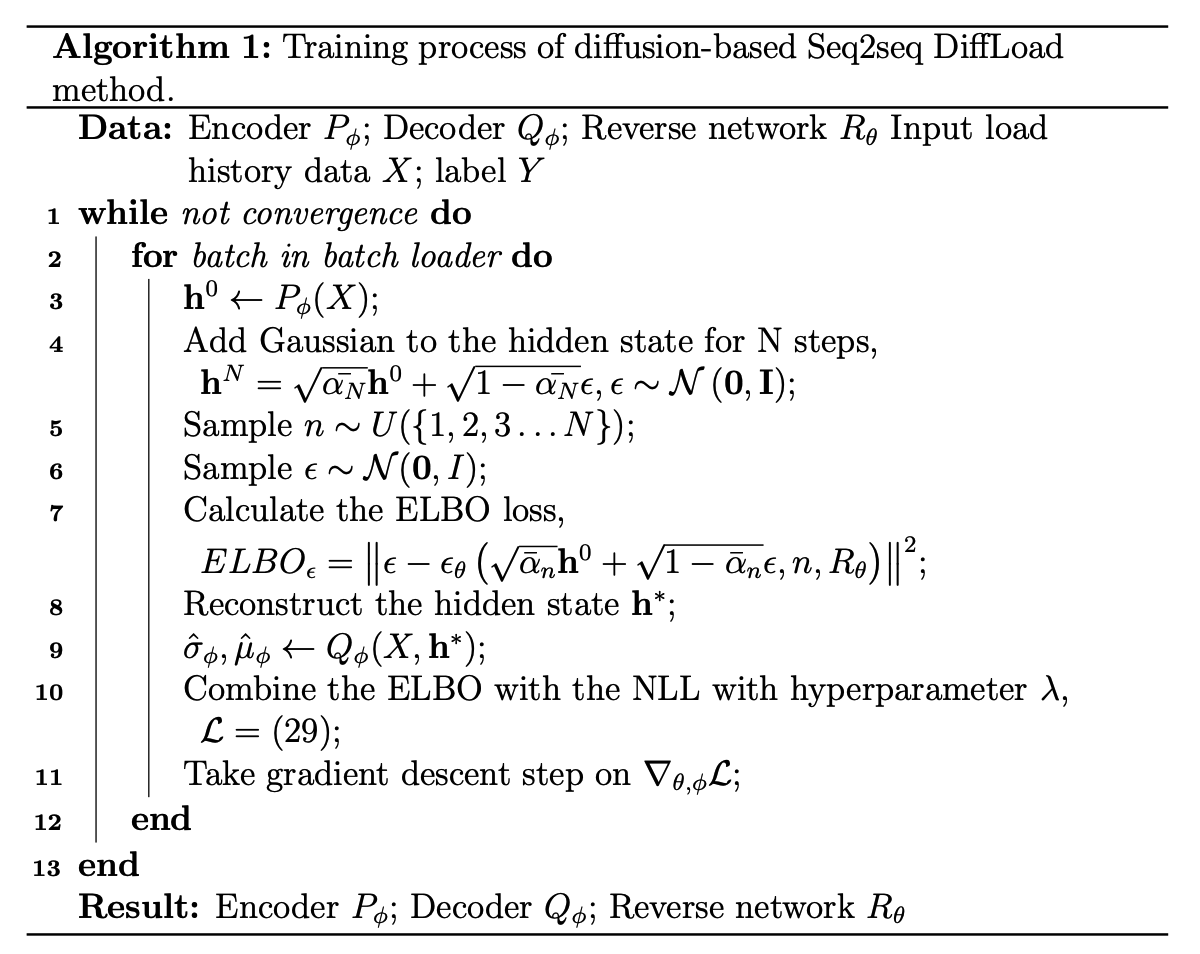
(3) Training & Inference

a) Training

Step 1) Obtain \(\hat{\mathbf{h}}_{t+1}^0\) after inputting the data into the diffusion-based Encoder.

• Concentrate the uncertainty of the model into the hidden state

Step 2) Put the \(\hat{\mathbf{h}}_{t+1}^0\) into the Decoder

• Output of the Decoder = parameter of the emission distribution
• Optimized by NLL

Loss function

• \(\mathcal{L}=\lambda E L B O-\log \hat{\sigma}_\phi+\log \left(\left(y-\hat{\mu}_\phi\right)^2+\hat{\sigma}_\phi^2\right)\).

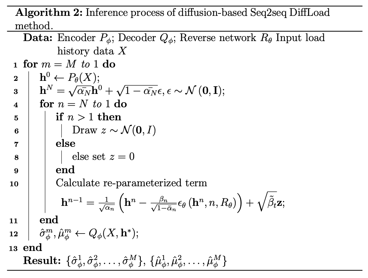
b) Inference

Infer for \(M\) times

Output of the Encoder undergoes the process of adding and removing noise

\(\rightarrow\) Randomness

Output of our model is the parameters : average

• \(\bar{\mu}=\frac{1}{M} \sum \hat{\mu}_\phi^i\).

c) Two kinds of uncertainties

1. Scale parameter
   • represent aleatoric uncertainty
2. Distnace btw upper / lower quantiles of location paramteres
   • obtained via multiple infferences
   • represent epistemic uncertainty

\(\begin{aligned} \bar{\sigma} & =\hat{\sigma}_\phi+\hat{\sigma}_\theta, \\ & =\frac{1}{M} \sum \hat{\sigma}_\phi^i+\left(q_u(\hat{\mu})-q_l(\hat{\mu})\right) \end{aligned}\).