ScoreGrad; Multivariate Probabilistic Time Series Forecasting with Continuous Energy-based Generative Models

ScoreGrad: Multivariate Probabilistic Time Series Forecasting with Continuous Energy-based Generative Models

Contents

1. Abstract
2. Introduction
3. Related Work
4. Score-based generative models
5. Method
6. Experiment

Abstract

Generative models in TS

• Many existing works can not be widely used because of the…
  • (1) constraints of functional form of generative models
  • (2) sensitivity to hyperparameters

ScoreGrad

• MTS probabilistic forecasting

• Continuous energy-based generative models

• Composed of ..
  • (1) TS feature extraction module
  • (2) Conditional stochastic differential equation based score matching module

• Prediction: by iteratively solving reverse-time SDE

  ( any numerical solvers for SDEs can be used for sampling )

• First continuous energy based generative model used for TS forecasting

1. Introuction

Limitations of previous works

• [3], [4] : can not model stochastic information in TS
• [5], [6] : can not model long range time dependencies

Generative models

• proved effective for sequential modeling
• WaveNet [7] : proposes TCN with dilation
• [8] : Combines transformer + masked autoregressive flow together
  • however, functional form the fothe models based on VAE & flow based models are constrained
• TimeGrad [9] : uses an energy-based generative model (EBM) which transforms data distribution to target distribution by slowly injecting noise

TimeGrad

• less restrictive on functional forms ( compared with VAE and flow based models )
• Limitations
  • (1) DDPM in TimeGrad is sensitive to the noise scales
  • (2) Number of steps used for noise injection needs to be carefully designed
  • (3) Sampling methods for generation process in DDPM can be further extended

ScoreGrad

• General framework for MTS forecasting based on continuous energy-based generative models

• DDPM = Discrete form of a stochastic differential equation (SDE)

  \(\rightarrow\) number of steps can be replaced by the interval of integration

  \(\rightarrow\) noise scales can be easily tuned by diffusion term in SDE

  \(\rightarrow\) conditional continuous energy based generative model + sequential modeling for forecasting!

2. Related Work

(1) MTS forecasting

pass

(2) Energy-based generative models

Energy-based models (EBMs)

• Un-normalized probabilistic models

• Compared with VAE & flow-based generative models…

  • EBMs directly estimate the unnormalized negative log-probability
  • Do not place a restriction on the tractability of the normalizing constants

  \(\rightarrow\) Much less restrictive in functional form

• Limitations: the unknown normalizing constant of EBMs will make training particularly difficult

Several methods for training EBMS

• (1) Maximum likelihood estimation based on MCMC
  • [26] : estimate the gradient of the log-likelihood with MCMC sampling methods, instead of directly computing the likelihood.
• (2) Score matching based methods
  • [28] : minimize a discrepancy between the gradient of the loglikelihood of data distribution and estimated distribution with Fisher divergence
    • optimization is computationally expensive!
• (3) Noise contrastive estimation
  • [29] : EBM can be learned by contrasting it with known density.

3. Score-based generative models

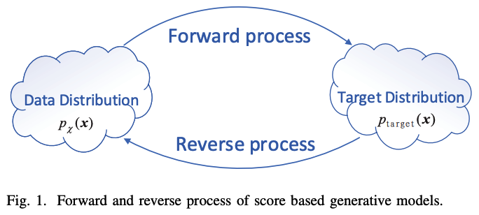
(1) Score matching models

\(\mathbf{x} \sim p_{\mathcal{X}}(\mathbf{x})\) : the distribution of a \(\mathrm{D}\) dim dataset

Score matching

• EBM which is proposed for learning “non-normalized” statistical models
• Aims to minimize the distance of the derivatives of the log-density function (= score) btw data and model distributions.

Although the density function of data distribution is unknown ..

Thanks to simple trick of partial integration.

\(\begin{aligned} L(\theta) &=\frac{1}{2} \mathbb{E}_{p_{\mathcal{X}}(\mathbf{x})} \mid \mid \nabla_{\mathbf{x}} \log p_\theta(\mathbf{x})-\nabla_{\mathbf{x}} \log p_{\mathcal{X}}(\mathbf{x}) \mid \mid _2^2 \\ & \quad=\mathbb{E}_{p_{\mathcal{X}}(\mathbf{x})}\left[\operatorname{tr}\left(\nabla_{\mathbf{x}}^2 \log p_\theta(\mathbf{x})\right)+\frac{1}{2} \mid \mid \nabla_{\mathbf{x}} \log p_\theta(\mathbf{x}) \mid \mid _2^2\right]+\mathrm{const} \end{aligned}\).

• \(\nabla_{\mathbf{x}} \log p_\theta(\mathbf{x})\) : score function

(2) Discrete score matching models

Two classes of EBMs that use various levels of noise to estimate score network

(1) Score matching with Langevin dynamics (SMLD)

• To improve score-based generative modeling by perturbing data with various levels of noise
• Trains a Noise Conditioned Score Network (NCSN) : \(s_\theta(\mathbf{x}, \sigma)\)
  • to estimate scores corresponding to all noise levels.
• Perturbation kernel : \(p_\sigma(\tilde{\mathbf{x}} \mid \mathbf{x}):=\mathcal{N}\left(\tilde{\mathbf{x}} ; \mathbf{x}, \sigma^2 \mathbf{I}\right)\).
  • noise sequence with ascending order \(\left\{\sigma_1, \sigma_2, \cdots, \sigma_N\right\}\), where…
    • \(\sigma_1\) is small enough that \(p_{\sigma_1}(\mathbf{x}) \approx p_{\mathcal{X}}(\mathbf{x})\)
    • \(\sigma_N\) is large enough that \(p_{\sigma_N}(\mathbf{x}) \approx \mathcal{N}\left(\mathbf{0}, \sigma_N^2 \mathbf{I}\right)\).

[ Training ]

Loss function: weighted sum of Denoising score matching objective

• \(L_\theta=\operatorname{argmin}_\theta \sum_{i=1}^N \mathbb{E}_{p_{\mathcal{X}}} \mathbb{E}_{p_{\sigma_i}}(\tilde{\mathbf{x}} \mid \mathbf{x})\left[ \mid \mid s_\theta\left(\tilde{\mathbf{x}}, \sigma_i\right)-\nabla_{\tilde{\mathbf{x}}} \log p_{\sigma_i}(\tilde{\mathbf{x}} \mid \mathbf{x}) \mid \mid _2^2\right]\).

[ Generation / Sampling ]

• Langevin MCMC is used for iterative sampling
• Number of iteration steps : \(\mathbf{M}\)
• Sampling process for \(p_{\sigma_i}(\mathbf{x})\) :
  • \(\mathbf{x}_i^m=\mathbf{x}_i^{m-1}+\epsilon_i s_\theta\left(\mathbf{x}_i^{m-1}, \sigma_i\right)+\sqrt{2 \epsilon_i} \mathbf{z}_i^m, m=1,2, \cdots, M\).
    • where \(\mathbf{z}_i^m \sim \mathcal{N}(\mathbf{0}, \mathbf{I}), \epsilon_i\) is the step size.
• Iteration sampling process is repeated for \(\mathrm{N}\) steps
  • \(N\) = number of different noises
  • \(\mathbf{x}_N^0 \sim\) \(\mathcal{N}\left(\mathbf{x} \mid \mathbf{0}, \sigma_N^2 \mathbf{I}\right)\) and \(\mathbf{x}_i^0=\mathbf{x}_{i+1}^M\) when \(i<N\).

(2) Denoising diffusion probabilistic models (DDPM)

[ Training ]

Forward process: \(p\left(\mathbf{x}_i \mid \mathbf{x}_{i-1}\right) \sim \mathcal{N}\left(\mathbf{x}_i ; \sqrt{1-\beta_i} \mathbf{x}_{i-1}, \beta_i \mathbf{I}\right)\)

\(\rightarrow\) \(p\left(\mathbf{x}_i \mid \mathbf{x}_0\right) \sim\) \(\mathcal{N}\left(\mathbf{x}_i ; \sqrt{\alpha_i} \mathbf{x}_0,\left(1-\alpha_i\right) \mathbf{I}\right)\),

• where \(\alpha_i=\prod_{k=1}^i\left(1-\beta_k\right)\).

Reverse process: \(q\left(\mathbf{x}_{i-1} \mid \mathbf{x}_i\right) \sim \mathcal{N}\left(\mathbf{x}_{i-1} ; \frac{1}{\sqrt{1-\beta_i}}\left(\mathbf{x}_i+\beta_i s_\theta\left(\mathbf{x}_i, i\right)\right), \beta_i \mathbf{I}\right)\)

Loss function: ELBO

• \(L(\theta)=\operatorname{argmin}_\theta \sum_{i=1}^N\left(1-\alpha_i\right) \mathbb{E}_{p_{\mathcal{X}}(\mathbf{x})} \mathbb{E}_{p_{\alpha_i}(\tilde{\mathbf{x}} \mid \mathbf{x})}\left[ \mid \mid s_\theta(\tilde{\mathbf{x}}, i)-\nabla_{\tilde{\mathbf{x}}} \log p_{\alpha_i}(\tilde{\mathbf{x}} \mid \mathbf{x}) \mid \mid _2^2\right]\).

[ Generation / Sampling ]

Based on the inverse Markov chain ( called ancestral sampling )

\(\mathbf{x}_{i-1}=\frac{1}{\sqrt{1-\beta_i}}\left(\mathbf{x}_i+\beta_i s_\theta\left(\mathbf{x}_i, i\right)\right)+\sqrt{\beta_i} \mathbf{z}_i\).

• where \(i=N, N-1, \cdots, 1\)

(3) Score matching with SDEs

Noise involvement process of above two methods can be modeled as numerical form of stochastic differential equations (SDE)

SDE: \(d \mathbf{x}=f\left(\mathbf{x}, t_s\right) d t_s+g\left(t_s\right) d \mathbf{w}\) ….. Eq (a)

• where \(\mathbf{w}\) represents a standard Wiener process

• \(f\left(\mathbf{x}, t_s\right)\) : drift coefficient

• \(g\left(t_s\right)\) : scalar function called diffusion coefficient

( [34] indicates that the reverse process of Eq (a) also satisfies a SDE as shown in Eq (b) )

\(d \mathbf{x}=\left[f\left(\mathbf{x}, t_s\right)-g\left(t_s\right)^2 \nabla_x \log p_{t_s}(\mathbf{x})\right] d t_s+g\left(t_s\right) d \mathbf{w}\) …… Eq (b)

\(\rightarrow\) SDE can be reversed if \(\nabla_{\mathbf{x}} \log p_t(\mathbf{x})\) at each intermediate time step is known!!!

Also, forward process of the above two models (1) & (2)

• (1) Discrete score matching models
• (2) DDPMs

can be treated as DISCRETE form of continuous-time SDEs

(1) Discrete score matching models: \(p_\sigma(\tilde{\mathbf{x}} \mid \mathbf{x}):=\mathcal{N}\left(\tilde{\mathbf{x}} ; \mathbf{x}, \sigma^2 \mathbf{I}\right)\)

• can be seen as DISCRETE version of process \(\left\{\mathbf{x}\left(t_s\right)\right\}_{t_s=0}^1\)

  such that \(d \mathbf{x}=\sqrt{\frac{d\left[\sigma^2\left(t_s\right)\right]}{d t_s}} d \mathbf{w}\)

  \(\rightarrow\) gives a process with exploding variance when \(t \rightarrow \infty\)

• called Variance Exploding (VE) SDE.

(2) DDPMs: \(p\left(\mathbf{x}_i \mid \mathbf{x}_{i-1}\right) \sim \mathcal{N}\left(\mathbf{x}_i ; \sqrt{1-\beta_i} \mathbf{x}_{i-1}, \beta_i \mathbf{I}\right)\)

• when \(N \rightarrow \infty\), Eq. 5 converges to

  \[d \mathbf{x}=-\frac{1}{2} \beta\left(t_s\right) \mathbf{x} d t_s+\sqrt{\beta\left(t_s\right)} d \mathbf{w}\]

• called Variance Preserving (VP) SDE

  • because the variance \(\boldsymbol{\Sigma}(t)\) is always bounded given \(\boldsymbol{\Sigma}(0)\).

4. Method

(1) Symbol and Problem formulation

MTS: \(\mathcal{X}=\left\{\mathbf{x}_1^0, \mathbf{x}_2^0, \cdots, \mathbf{x}_T^0\right\}\),

Prediction tasks for MTS: estimate \(q_{\mathcal{X}}\left(\mathbf{x}_{t_0: T}^0 \mid \mathbf{x}_{1: t_0-1}^0, \mathbf{c}_{1: T}\right)\),

• where \(\mathbf{c}_{1: T}\) represents covariates ( known for all time points )

Iterative forecasting strategy: \(q_{\mathcal{X}}\left(\mathbf{x}_{t_0: T}^0 \mid \mathbf{x}_{1: t_0-1}^0, \mathbf{c}_{1: T}\right)=\prod_{t=t_0}^T q_{\mathcal{X}}\left(\mathbf{x}_t^0 \mid \mathbf{x}_{t-1}^0, \mathbf{c}_{1: T}\right)\)

(2) Model Architecture

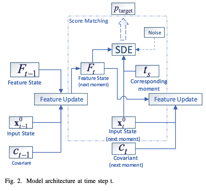
Two modules at each time step

• (1) Time series feature extraction module
• (2) Conditional SDE based score matching module

a) TS feature extraction module

Goal: get a feature \(\mathbf{F}_t\) of historical time series data until \(t-1\)

Update function : \(\mathbf{F}_t=R\left(\mathbf{F}_{t-1}, \mathbf{x}_{t-1}, \mathbf{c}_{t-1}\right)\)

• ex) RNN: \(F_t\) corresponds to hidden state \(\mathbf{h}_{t-1}\)
• ex) TCN, attention: \(\mathbf{F}_t\) is a vector that represents the features learned by historical data and covariates

Iterative forecasting strategy = conditional prediction problem

• \(\prod_{t=t}^T q_{\mathcal{X}}\left(\mathbf{x}_t^0 \mid \mathbf{x}_{t-1}^0, \mathbf{c}_{1: T}\right)=\prod_{t=t}^T p_\theta\left(\mathbf{x}_t^0 \mid \mathbf{F}_t\right)\).

  • \(\theta\) : learnable parameters of \(R\)

    ( use RNN for ScoreGrad )

b) Conditional SDE based score matching module

\(\mathbf{F}_t\) : used as a conditioner for SDE based score matching models at each time step.

Initial state distribution : \(p\left(\mathbf{x}_t^0 \mid \mathbf{F}_t\right)\)

Forward evolve process :

• \(d \mathbf{x}=f\left(\mathbf{x}, t_s\right) d t_s+g\left(t_s\right) d \mathbf{w}\).

Reverese timeSDE:

• \(d \mathbf{x}_t=\left[f\left(\mathbf{x}_t, t_s\right)-g\left(t_s\right)^2 \nabla_x \log p_{t_s}\left(\mathbf{x}_t \mid \mathbf{F}_t\right)\right] d t_s+g\left(t_s\right) d \mathbf{w}\).

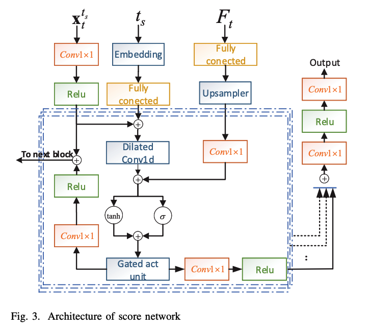
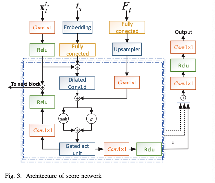
c) Conditional score network

( Inspired by WaveNet & DiffWave )

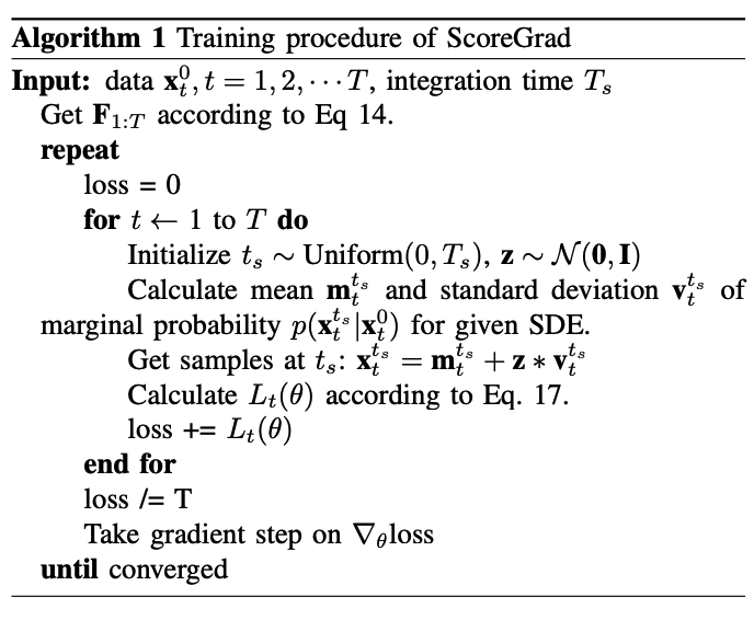
d) Training

\[\begin{aligned} & L_t(\theta)=\operatorname{argmin}_\theta \mathbb{E}_{t_s}\left(\lambda\left(t_s\right) \mathbb{E}_{\mathbf{x}_t^0} \mathbb{E}_{\mathbf{x}_t^{t_s} \mid \mathbf{x}_t^0}\right. \\ & \left.\quad\left[ \mid \mid s_\theta\left(\mathbf{x}_t^{t_s}, \mathbf{F}_t, t_s\right)-\nabla_{\mathbf{x}_t^{t_s}} \log p_{0 t_s}\left(\mathbf{x}_t^{t_s} \mid \mathbf{x}_t^0\right) \mid \mid _2^2\right]\right) \end{aligned}\]

\(L(\theta)=\frac{1}{T} \sum_{t=1}^T L_t(\theta)\).

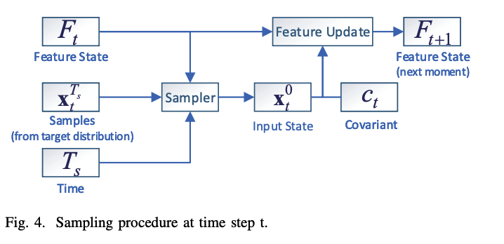
e) Prediction

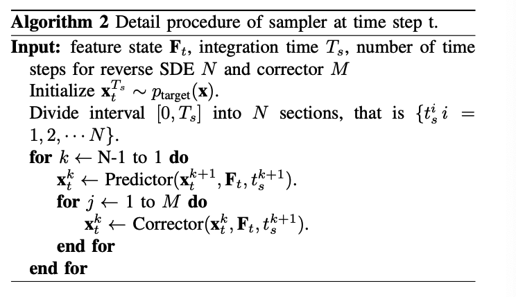
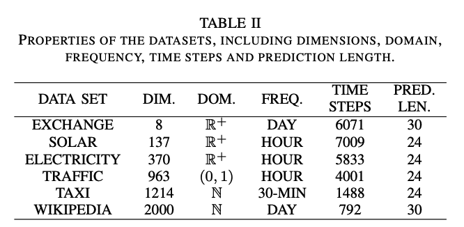
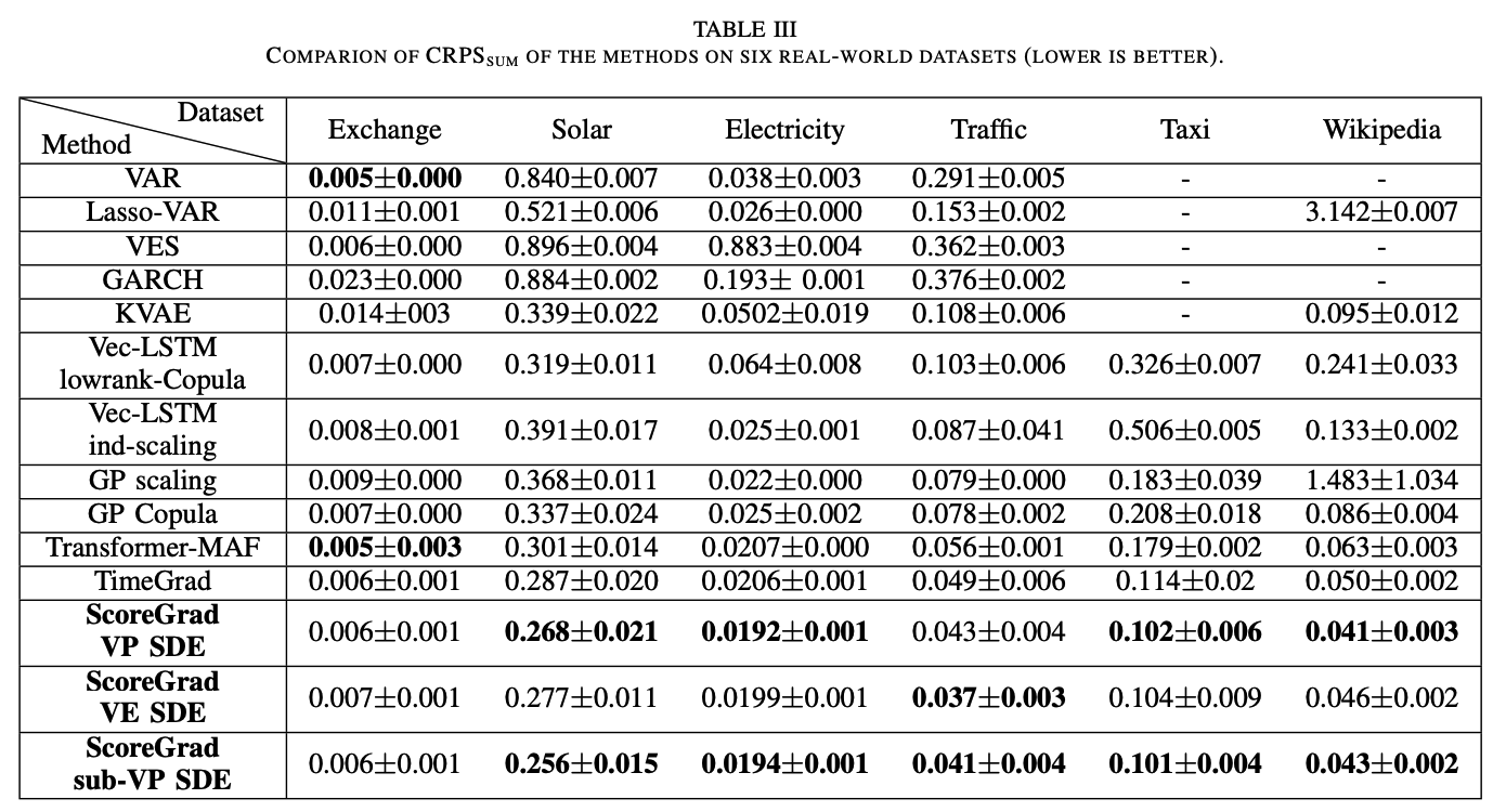
5. Experiment