Diffusion Convolutional Recurrent Neural Network : Data-driven Traffic Forecasting
Contents
- Abstract
- Introduction
- Methodology
- Traffic Forecasting Problem
- Spatial Dependency Modeling
- Temporal Dynamics Modeling
0. Abstract
Traffic forecasting is challenging, due to..
- 1) complex spatial dependency
- 2) non-linear temporal dynamics
- 3) difficulty of long-term forecasting
Introduce DCRNN (Diffusion Convolutional Recurrent Neural Network)
- for “traffic forecasting”
- incorporates both (1) spatial & (2) temporal dependency in traffic flow
DCRNN captures…
- 1) “spatial dependency” : using the “bidirectional RW” on graph
- 2) “temporal dependency” : using the “enc-dec” architecture, with “scheduled sampling”
1. Introduction
Difficulty of traffic forecasting
ex) road 1 & 3 : close in Euclidean space, but very different behaviors
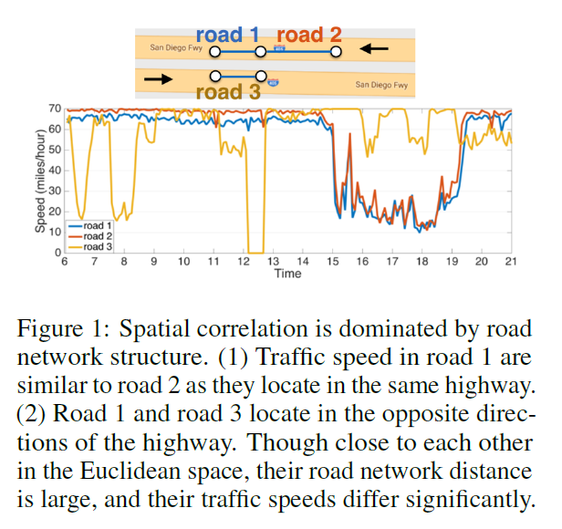
\(\rightarrow\) spatial structure in traffic is non-Euclidean & directional
DCRNN
-
represent “pair-wise spatial correlations” between traffic sensors, using a “directed graph”
- 1) nodes : sensors
- 2) edge : proximity between sensor pairs
-
model the dynamics of the traffic flow as a “diffusion process”
\(\rightarrow\) propose the diffusion convolution to capture “spatial dependency”
-
integrates
- 1) diffusion convolution
- 2) seq2seq
- 3) scheduled sampling
2. Methodology
(1) Traffic Forecasting Problem
Goal : predict the future traffic speed, given traffic flow from \(N\) correlated sensors
Graph ( Sensor Network )
-
Weighted directed graph : \(\mathcal{G}=(\mathcal{V}, \mathcal{E}, \boldsymbol{W})\)
-
\(\mathcal{V}\) : set of nodes ( \(\mid \mathcal{V} \mid=N\) )
-
\(\mathcal{E}\) : set of edges
-
\(\boldsymbol{W} \in \mathbb{R}^{N \times N}\) : weighted adjacency matrix
( representing the nodes proximity … e.g., a function of their road network distance )
-
-
Traffic flow observed on \(\mathcal{G}\) : \(\boldsymbol{X} \in \mathbb{R}^{N \times P}\)
- \(P\) : # of features ( ex. velocity, volume … )
- \(\boldsymbol{X}^{(t)}\) : graph signal observed at time \(t\)
-
goal : learn function \(h(\cdot)\), where…
- \(\left[\boldsymbol{X}^{\left(t-T^{\prime}+1\right)}, \cdots, \boldsymbol{X}^{(t)} ; \mathcal{G}\right] \stackrel{h(\cdot)}{\longrightarrow}\left[\boldsymbol{X}^{(t+1)}, \cdots, \boldsymbol{X}^{(t+T)}\right]\).
(2) Spatial Dependency Modeling
model the spatial dependency,
by relating “traffic flow” to a “diffusion process”
Diffusion process
Notation
-
1) random walk on \(\mathcal{G}\)
-
2) restart probability \(\alpha \in [0,1]\)
-
3) state transition matrix \(\boldsymbol{D}_{O}^{-1} \boldsymbol{W}\)
- \(D_{O}=\operatorname{diag}(W 1)\) = out-degree diagonal matrix
- converges to a stationary distribution \(\mathcal{P} \in \mathbb{R}^{N \times N}\)
- \(\mathcal{P}_{i,:} \in \mathbb{R}^{N}\) ( \(i\) th row ) = likelihood of diffusion from node \(v_{i} \in \mathcal{V}\)
- can be calculated in closed-form, \(\mathcal{P}=\sum_{k=0}^{\infty} \alpha(1-\alpha)^{k}\left(\boldsymbol{D}_{O}^{-1} \boldsymbol{W}\right)^{k}\)
( in practice, use finite \(K\)-step truncation )
Diffusion Convolution
Diffusion Convolution Operation…
- over a graph signal \(\boldsymbol{X} \in \mathbb{R}^{N \times P}\)
- and a filter \(f_{\boldsymbol{\theta}}\)
\(\boldsymbol{X}_{:, p} \star_{\mathcal{G}} f_{\boldsymbol{\theta}}=\sum_{k=0}^{K-1}\left(\theta_{k, 1}\left(\boldsymbol{D}_{O}^{-1} \boldsymbol{W}\right)^{k}+\theta_{k, 2}\left(\boldsymbol{D}_{I}^{-1} \boldsymbol{W}^{\boldsymbol{\top}}\right)^{k}\right) \boldsymbol{X}_{:, p} \quad \text { for } p \in\{1, \cdots, P\}\).
- \(\boldsymbol{\theta} \in \mathbb{R}^{K \times 2}\) = parameters for the filter
- \(\boldsymbol{D}_{O}^{-1} \boldsymbol{W}, \boldsymbol{D}_{I}^{-1} \boldsymbol{W}^{\top}\) = transition matrices of the diffusion process & reverse one
Diffusion Convolutional Layer
- maps \(P\)-dim features to \(Q\)-dim outputs
- Input : \(\boldsymbol{X} \in \mathbb{R}^{N \times P}\)
- Output : \(\boldsymbol{H} \in \mathbb{R}^{N \times Q}\)
- \(\boldsymbol{H}_{:, q}=\boldsymbol{a}\left(\sum_{p=1}^{P} \boldsymbol{X}_{:, p} \star \mathcal{G} f_{\Theta_{q, p, i,:}}\right) \quad \text { for } q \in\{1, \cdots, Q\}\).
(3) Temporal Dynamics Modeling
use GRU ( + replace matrix multiplication in GRU with “diffusion convolution” )
\(\rightarrow\) DCGRU (Diffusion Convolutional Gated Recurrent Unit)
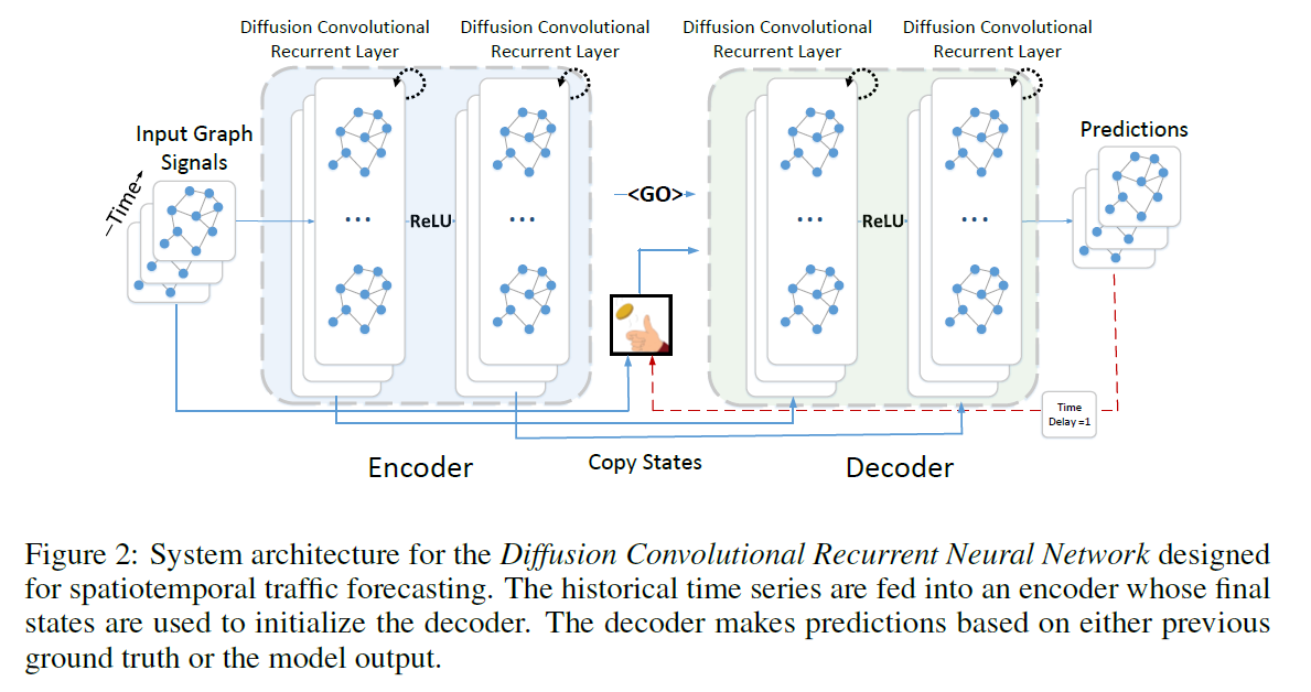
in multi-step ahead forecasting, use “seq2seq”
-
both ENC & DEC are “DCGRU”
-
scheduled sampling : decoder ~
-
( training ) generates predictions, given (a) previous ground truth observation or (b) predictions
-
with prob \(\epsilon_i\) : (a)
-
with prob \(1- \epsilon_i\) : (b)
( during the training process, \(\epsilon_i\) gradually decreases to \(0\) )
-
-
( testing ) generates predictions, given (a) predictions
-