(paper) Graph WaveNet for Deep Spatial-Temporal Graph Modeling

Graph WaveNet for Deep Spatial-Temporal Graph Modeling

Contents

1. Abstract
2. Introduction
3. Related Works
   1. GCN
   2. Spatial-temporal Graph Networks
4. Methodology
   1. Problem Definition
   2. GCN layer
   3. TCN layer
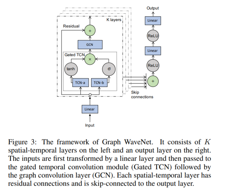
   4. Framework of Graph WaveNet

0. Abstract

Spatial-temporal graph modeling : analyze..

• 1) spatial relations
• 2) temporal trends

Problem :

• 1) explicit graph structure “does not necessarily reflect the true dependency”
• 2) existing methods are ineffective to capture temporal trends
  • RNNs, CNNs : can not capture LONG-range temporal sequences

Graph Wavenet

• (1) develop a novel adaptive dependency matrix
• (2) stacked dilated 1D conv ( able to handle very LONG sequences )

1. Introduction

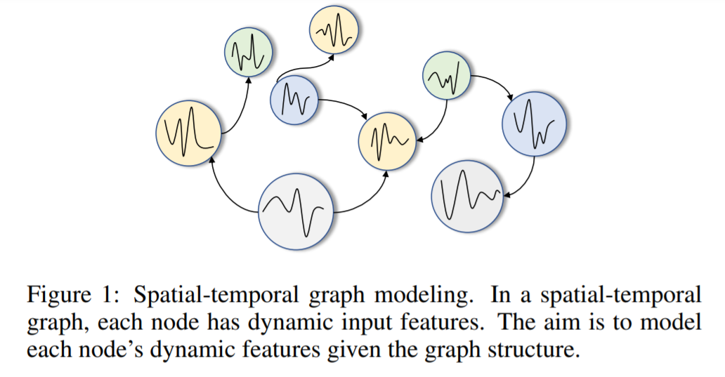
Spatial-temporal graph modeling

• aims to model the “dynamic node-level inputs”

  by assuming “inter-dependency between nodes”

• ex ) traffic speed forecasting
• basic assumption :
  • node’s future information is conditioned on..
    • 1) its historical info
    • 2) neighbors’ historical info

• key point :

  • how to capture SPATIAL and TEMPORAL dependencies

Recent works : 2 directions

• 1) integrate GCN into RNN
• 2) integrate GCN into CNN

Shortcomings of 2 approaches

• 1) assumes that “graph structure reflects genuine dependency”

  \(\rightarrow\) not always the case

• 2) ineffective to learn temporal dependencies

Graph WaveNet

• address the 2 shortcomings
• 2 key points
  • 1) self-adaptive adjacency matrix
  • 2) stacked dilated causal convolutions

2. Related Works

(1) GCN

• building blocks for learning graph-structured data
• widely used in..
  • node embedding / node classification / graph classification / link prediction / node clustering
• 2 main streams of GCN
  • 1) Spectral-based approaches
    • smooth a node’s input signals, using graph spectral filters
  • 2) Spatial-based appraoches
    • extract node’s high-level representation, by aggregating feature info from neighbors
    • (usually) adjacency matrix is considered as prior & fixed throughout training

(2) Spatial-temporal Graph Networks

2 directions

• 1) RNN-based : inefficient for long sequences
• 2) CNN-based : efficient, but have to stack many layers

3. Methodology

Two building blocks of Graph WaveNet

• 1) GCN (Graph Convolutional Layer)
• 2) TCN (Temporal Convolutional Layer)

\(\rightarrow\) work together to capture the “spatial-temporal dependencies”

(1) Problem Definition

Notation

• graph : \(G=(V, E)\)

• adjacency matrix : \(\mathbf{A} \in \mathbf{R}^{N \times N}\)

• ( at each time step \(t\) )

  dynamic feature of \(G\) : \(\mathbf{X}^{(t)} \in \mathbf{R}^{N \times D} .\) ( = graph signals )

Goal : \(\left[\mathbf{X}^{(t-S): t}, G\right] \stackrel{f}{\rightarrow} \mathbf{X}^{(t+1):(t+T)}\).

• given (1) graph \(G\) & (2) historical \(S\) step graph signals,
• predict next \(T\) step graph signals

(2) GCN layer

extract a node’s features, given structural information

Graph Convolution Layer : \(\mathbf{Z}=\tilde{\mathbf{A}} \mathbf{X} \mathbf{W}\)

• \(\tilde{\mathbf{A}} \in \mathbf{R}^{N \times N}\) : normalized adjacency matrix ( with self-loops )
• \(\mathbf{X} \in \mathbf{R}^{N \times D}\) : input signals
• \(\mathbf{Z} \in \mathbf{R}^{N \times M}\) : output
• \(\mathbf{W} \in \mathbf{R}^{D \times M}\) : model parameter matrix

Diffusion Convolution Layer : \(\mathbf{Z}=\sum_{k=0}^{K} \mathbf{P}^{k} \mathbf{X} \mathbf{W}_{\mathbf{k}}\)

• effective in “spatial-temporal modeling”
• modeled the diffusion process of graph signals with \(K\) finite steps

• \(\mathbf{P}^{k}\) : the power series of the transition matrix

• ( if directed ) \(\mathbf{Z}=\sum_{k=0}^{K} \mathbf{P}_{f}^{k} \mathbf{X W}_{k 1}+\mathbf{P}_{b}^{k} \mathbf{X} \mathbf{W}_{k 2}\)

Self-adaptive Adjacency Matrix : \(\tilde{\mathbf{A}}_{a d p}\)

\(\tilde{\mathbf{A}}_{a d p}=\operatorname{Soft} \operatorname{Max}\left(\operatorname{ReLU}\left(\mathbf{E}_{1} \mathbf{E}_{2}^{T}\right)\right)\).

• does not require any prior knowledge

• let the model discover hidden spatial dependencies

• Notation

  • \(\mathbf{E} 1\) : source node embedding

  • \(\mathbf{E} 2\) : target node embedding

    ( by multiplying both, derive the “spatial dependency weights between 2 nodes” )

• this \(\tilde{\mathbf{A}}_{a d p}\) can be considered as “transition matrix” of hidden diffusion process

Proposal :

• (if graph structure : available)
  • \[\mathbf{Z}=\sum_{k=0}^{K} \mathbf{P}_{f}^{k} \mathbf{X} \mathbf{W}_{k 1}+\mathbf{P}_{b}^{k} \mathbf{X} \mathbf{W}_{k 2}+\tilde{\mathbf{A}}_{a p t}^{k} \mathbf{X} \mathbf{W}_{k 3} .\]
• (if graph structure : unavailable)
  • \(\mathbf{Z}=\sum_{k=0}^{K} \tilde{\mathbf{A}}_{a p t}^{k} \mathbf{X} \mathbf{W}_{k}\).

(3) TCN layer

adopt “dilated causal convolution”

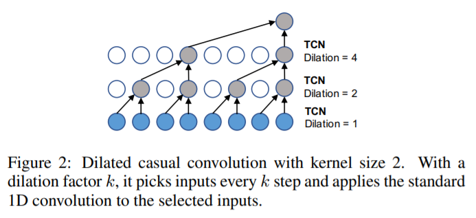
Gated TCN

• simple version : \(\mathbf{h}=g\left(\boldsymbol{\Theta}_{1} \star \mathcal{X}+\mathbf{b}\right) \odot \sigma\left(\mathbf{\Theta}_{2} \star \mathcal{X}+\mathbf{c}\right)\).
• use this to learn “complex temporal dependencies”

(4) Framework of Graph WaveNet