
Multivariate Time Series Forecasting with Transfer Entropy Graph (2020, 5)
Contents
-
Abstract
-
Introduction
-
Preliminaries
- Neural Granger Causality
- Graph Neural Network
-
Methodology
- Problem Formulation
-
Causality Graph Structure with Transfer Entropy
- Feature Extraction of Multiple Receptive Fields
- Node Embedding based on Causality Matrix
Abstract
most methods :
-
assume that predicted value of single variable is affected by ALL other variables
\(\rightarrow\) ignore the causal relationship among variables
propose CauGNN (graph neural network with Neural Granger Causality)
- node = each variable
- edge = causal relationship between variables
CNN filters with different perception scales are used ( for feature extraction )
1. Introduction
LSTNet
- encodes short-term local information into low-dim vector, using 1d-CNN
- decode the vectors through RNN
\(\rightarrow\) but, existing models cannot model the pairwise causal dependencies among MTS explicitly
G-causality ( Granger Causality Analysis )
- quantitative characterization of TS causality
- but, cannot well handle non-linear relationships
Transfer Entropy (TE)
- causal analysis, which can deal with non-linear cases
CauGNN
-
proposed method
-
1) after pairwise TE is calculated, TF matrix can be obtained
\(\rightarrow\) used as “adjacency matrix”
-
2) CNN filters with different perception scale
\(\rightarrow\) for TS feature extraction
-
3) GNN for embedding & forecasting
[ Contributions ]
-
consider MTS as a graph structure with causality
-
use transfer entropy to extract causality
& construct TE graph
2. Preliminaries
(1) Neural Granger Causality
Granger Causality
if addition of historical info of variable \(i\) improves the prediction of variable \(j\),
\(\rightarrow\) variable \(i\) is the cause of variable \(j\)
Granger Causality vs Neural Granger Causality
- Granger Causality
- traditional linear model
- use the AR model for prediction
- Neural Granger Causality
- use DL & regularization for non-linearity
Neural Granger Network
consists of 2 parts
- 1) variable selection module
- 2) prediction module
a) variable selection module
- FC layer ( input = historical TS )
- select key variables by group Lasso regularization
- if specific group is not significant \(\rightarrow\) will be zero (0)
b) prediction module
- MLP or LSTM
- general prediction method
Objective function
- \(\min _{W} \sum_{t=K}^{T}\left(x_{i t}-g_{i}\left(\boldsymbol{x}_{(t-1):(t-K)}\right)\right)^{2}+\lambda \sum_{j=1}^{p} \mid \mid \left(\boldsymbol{W}_{: j}^{\mathbf{1 1}}, \ldots, \boldsymbol{W}_{: j}^{\mathbf{1} K}\right) \mid \mid _{F}\).
(2) Graph Neural Network
most of GNN approaches fit within the framework of “neural message passing”
GNN can be viewed as… message passing algorithm,
where node representations are iteratively computed from the features of neighbor nodes
( using differentiable aggregation function )
GCN
- can be regarded as…
- 1) approximation of spectral-domain convolution of graph signals
- 2) sampling & aggregating of neighborhood information
GraphSAGE
- enabling training in batches
GIN (Graph Isomorphism Network)
- enable more complex forms of aggregation
GAT
- attending over the neighbors via self-attention
3. Methodology
(1) Problem Formulation
- observed TS : \(\boldsymbol{X}_{n}=\left[\boldsymbol{x}_{1}, \boldsymbol{x}_{\boldsymbol{2}}, \ldots, \boldsymbol{x}_{t}\right]\)
- \(\boldsymbol{x}_{\boldsymbol{i}} \in \mathbb{R}^{n}(i=\) \(1, \ldots, n)\)
- \(n\) : number of variables
- goal : predict \(\boldsymbol{x}_{t+h}\)
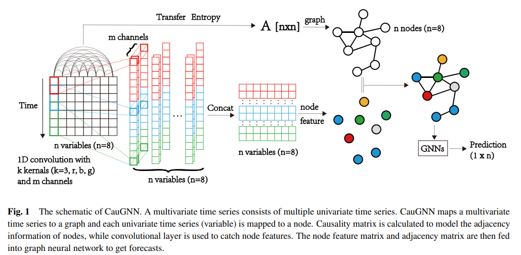
(2) Causality Graph Structure with Transfer Entropy
(Information) Entropy : \(H(\boldsymbol{X})=-\sum p(x) \log _{2} p(x)\).
- larger entropy \(\rightarrow\) more information
Conditional Entropy : \(H(\boldsymbol{X} \mid \boldsymbol{Y})=-\sum \sum p(x, y) \log _{2} p(x \mid y)\)
- information about \(\mathbf{X}\), given \(\mathbf{Y}\) is known
TE of variables \(\mathbf{Y}\) to \(\mathbf{X}\) :
\(\begin{aligned} T_{\boldsymbol{Y} \rightarrow \boldsymbol{X}}=& \sum p\left(x_{t+1}, \boldsymbol{x}_{t}^{(k)}, \boldsymbol{y}_{t}^{(l)}\right) \log _{2} p\left(x_{t+1} \mid \boldsymbol{x}_{t}^{(k)}, \boldsymbol{y}_{t}^{(l)}\right) \\ &-\sum p\left(x_{t+1}, \boldsymbol{x}_{t}^{(k)}\right) \log _{2} p\left(x_{t+1} \mid \boldsymbol{x}_{t}^{(k)}\right) \\ =& \sum p\left(x_{t+1}, \boldsymbol{x}_{t}^{(k)}, \boldsymbol{y}_{t}^{(l)}\right) \log _{2} \frac{p\left(x_{t+1} \mid \boldsymbol{x}_{t}^{(k)}, \boldsymbol{y}_{t}^{(l)}\right)}{p\left(x_{t+1} \mid \boldsymbol{x}_{t}^{(k)}\right)} \\ =& H\left(\boldsymbol{X}_{t+1} \mid \boldsymbol{X}_{t}\right)-H\left(\boldsymbol{X}_{t+1} \mid \boldsymbol{X}_{t}, \boldsymbol{Y}_{t}\right) \end{aligned}\).
- “increase in information of \(X\)“, when \(Y\) changes from “unknown to known”
- assymetric
Causal relationship between \(X\) & \(Y\)
- \(T_{\boldsymbol{X}, \boldsymbol{Y}}=T_{\boldsymbol{X} \rightarrow \boldsymbol{Y}}-T_{\boldsymbol{Y} \rightarrow \boldsymbol{X}}\).
- \(T_{\boldsymbol{X}, \boldsymbol{Y}} > 0\) : \(\boldsymbol{X}\) is the cause of \(\boldsymbol{Y}\)
- \(T_{\boldsymbol{X}, \boldsymbol{Y}} < 0\) : \(\boldsymbol{Y}\) is the cause of \(\boldsymbol{X}\)
use neural granger to capture causality
-
causality matrix \(\mathbf{T}\) of mts \(X_n\) can be formulated with…
\(t_{i j}=\left\{\begin{array}{lc} T_{\boldsymbol{x}_{i}, \boldsymbol{x}_{j}}, & T_{\boldsymbol{x}_{i}, \boldsymbol{x}_{j}}>c \\ 0, & \text { otherwise } \end{array}\right.\).
\(\rightarrow\) use as “adjacency matrix of MTS graph”
(3) Feature Extraction of Multiple Receptive Fields
necessary to consider trend & seasonality
\(\rightarrow\) thus, need to extract the features of TS in units of multiple certain periods
\(\rightarrow\) use multiple CNN filters
- \(\boldsymbol{h}_{\boldsymbol{i}}=\operatorname{ReLU}\left(\boldsymbol{W}_{\boldsymbol{i}} * \boldsymbol{x}+\boldsymbol{b}_{\boldsymbol{i}}\right), \boldsymbol{h}=\left[\boldsymbol{h}_{\mathbf{1}} \oplus \boldsymbol{h}_{\mathbf{2}} \oplus \ldots \oplus \boldsymbol{h}_{\boldsymbol{p}}\right] .\).
(4) Node Embedding based on Causality Matrix
after feature extraction,
input MTS is converted into feature matrix \(\boldsymbol{H} \in \mathbb{R}^{n \times d}\)
- feature matrix with \(n\) nodes
adjacency of nodes is determined by causality matrix \(T\)
inspired by k-GNNs
-
only perform information fusion between “neighbors”
( ignore information of non-neighbors )
Forward-pass update :
- \(\boldsymbol{h}_{i}^{(l+1)}=\sigma\left(\boldsymbol{h}_{i}^{(l)} \boldsymbol{W}_{1}^{(l)}+\sum_{j \in N(i)} \boldsymbol{h}_{j}^{(l)} \boldsymbol{W}_{2}^{(l)}\right)\).