DeepHit

DeepHit : A Deep Learning Approach to Survival Analysis with Competing Risks

Contents

1. Abstract

2. Introduction
3. Survival Analysis
   1. Survival Data
   2. Model Description
   3. Loss Function

0. Abstract

Relationship between “covariates” & “survival times (=times-to-event)”

Previous works :

• assume a specific form for the underlying stochastic process

DeepHit

• 1) makes no assumptions!
• 2) allows for possibility that the relationship between covariates & risks change over time
• 3) handles competing risks

1. Introduction

Survival Analysis is further applied to…

• “discovering risk factors” affecting the survival
• “comparison among risks” of different subjects

DeepHit

• no assumptions about the form of underlying stochastic process
• learns the distribution of first hitting times DIRECTLY
• both cases OK
  • 1) single risk ( cause )
  • 2) multiple competing risks ( causes )
• architecture
  • [1] single shared sub-network
  • [2] family of cause-specific sub-networks
• loss function
  • [1] survival times
  • [2] relative risks

2. Survival Analysis

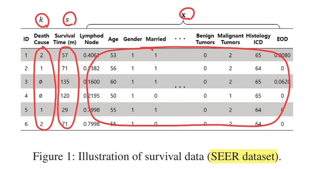
(1) Survival Data

3 pieces of information

• 1) observed covariates
• 2) time elapsed, since covariates were first collected
• 3) label indicating type of event

Settings :

• time : discrete
• time horizon : finite ( ex. no longer live than 100 years! )

Notation

• time set : \(\mathcal{T}=\left\{0, \ldots, T_{\max }\right\}\)
• possible events : \(\mathcal{K}=\{\varnothing, 1, \cdots, K\}\)
  • \(\varnothing\) : “Right-censoring” event
• assumption : “exactly ONE event occurs for each patient”
• triple : \((\mathbf{x}, s, k)\)
  • 1) covariate : \(\mathbf{x} \in X\)
  • 2) time at which the (unique) event or censoring occurred : \(s\)
  • 3) event or censoring that occurred at time \(s\) : \(k \in \mathcal{K}\)
• dataset : \(\mathcal{D}=\left\{\left(\mathbf{x}^{(i)}, s^{(i)}, k^{(i)}\right)\right\}_{i=1}^{N}\)

Goal

• for each tuple \(\left(\mathbf{x}^{*}, s^{*}, k^{*}\right)\) with \(k^{*} \neq \varnothing\),

• predict true probability \(P\left(s=s^{*}, k=k^{*} \mid \mathbf{x}=\mathbf{x}^{*}\right)\)

  ( find estimates \(\hat{P}\) of true probabilities)

(2) Model Description

Goal : learn \(\hat{P}\) ( = estimate of “joint distn of (1) first hitting time & (2) competing events “)

DeepHit : multi-task network

• 1) \(1\) shared sub-network
• 2) \(K\) cause-specific sub-networks

DeepHit vs MTL

• 1) SINGLE softmax layer
• 2) Residual Connection

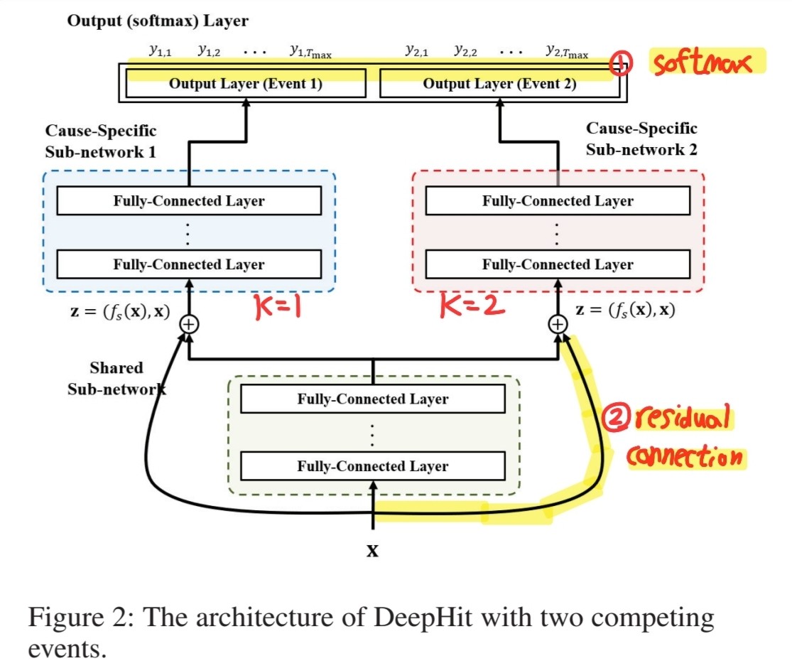
Cause-specific sub-network

Input : pairs \(\mathbf{z}=\left(f_{s}(\mathbf{x}), \mathbf{x}\right)\)

Output : \(f_{c_{k}}(\mathbf{z})\)

• (= probability of the first hitting time of a specific cause \(k\) )

Totality of these outputs :

• joint probability distn on (1) first hitting time & (2) event
• output of softmax layer :
  • \(\mathbf{y}=\left[y_{1,1}, \cdots, y_{1, T_{\max }}, \cdots, y_{K, 1}, \cdots, y_{K, T_{\max }}\right]\).

(cause-specific) Cumulative Incidence Function (CIF)

• probability that event \(k^{*} \in \mathcal{K}\),

  occurs on/before time \(t^{*}\)

  conditional on covariates \(\mathbf{x}^{*}\)

• \(\begin{aligned} F_{k^{*}}\left(t^{*} \mid \mathbf{x}^{*}\right) &=P\left(s \leq t^{*}, k=k^{*} \mid \mathbf{x}=\mathbf{x}^{*}\right) \\ &=\sum_{s^{*}=0}^{t^{*}} P\left(s=s^{*}, k=k^{*} \mid \mathbf{x}=\mathbf{x}^{*}\right) \end{aligned}\).

• true CIF is not known

  \(\rightarrow\) use estimated CIF, \(\hat{F}_{k^{*}}\left(s^{*} \mid \mathbf{x}^{*}\right)=\sum_{m=0}^{s^{*}} y_{k, m}^{*}\)

(3) Loss Function

\(\mathcal{L}_{\text {Total }}=\mathcal{L}_{1}+\mathcal{L}_{2}\).

• \(\mathcal{L_1}\) : log-likelihood of the joint distribution of the first hitting time and event
• \(\mathcal{L_2}\) : combination of cause-specific ranking loss functions.

Term 1 : \(\mathcal{L_1}\)

\(\begin{aligned} \mathcal{L}_{1}=-& \sum_{i=1}^{N}\left[\mathbb{1}\left(k^{(i)} \neq \varnothing\right) \cdot \log \left(y_{k^{(i)}, s^{(i)}}^{(i)}\right)\right. \left.+\mathbb{1}\left(k^{(i)}=\varnothing\right) \cdot \log \left(1-\sum_{k=1}^{K} \hat{F}_{k}\left(s^{(i)} \mid \mathbf{x}^{(i)}\right)\right)\right] \end{aligned}\).

• total : \(K\) competing risks

• patients

  • (not censored) : captures both the “event” & “time” the event occured
  • (censored) : captures “time” censored

Term 2 : \(\mathcal{L_2}\)

\(\mathcal{L}_{2}=\sum_{k=1}^{K} \alpha_{k} \cdot \sum_{i \neq j} A_{k, i, j} \cdot \eta\left(\hat{F}_{k}\left(s^{(i)} \mid \mathbf{x}^{(i)}\right), \hat{F}_{k}\left(s^{(i)} \mid \mathbf{x}^{(j)}\right)\right)\).

\(A_{k, i, j} \triangleq \mathbb{1}\left(k^{(i)}=k, s^{(i)}<s^{(j)}\right)\).

• estimated CIFs calculated at different times

• to fine-tune network to each “cause-specific estimated CIF”

• penalizes incorrect ordering of pairs

• utilize ranking loss function

  • adapts the idea of concordance

    ( = patient who dies at \(s\) should have higher risk at time \(s\) , than a patient who survived longer than \(s\) )

Notation

• coefficients \(\alpha_{k}\) : chosen to trade off ranking losses of the \(k\)-th competing event
  • assume here that the coefficients \(\alpha_{k}\) are all equal (i.e. \(\alpha_{k}=\alpha\) )
• \(\eta(x, y)\) : convex loss function
  • use the loss function \(\eta(x, y)=\exp \left(\frac{-(x-y)}{\sigma_{\text {. }}}\right) .\)