(paper) A Transformer-based Framework for Multivariate Time Series Representation Learning

A Transformer-based Framework for Multivariate Time Series Representation Learning (2020,22)

Contents

1. Abstract
2. Introduction
3. Related Works
4. Methodology
   1. Base Model
   2. Regression & Classification
   3. Unsupervised Pre-training

0. Abstract

• TRANSFORMER for UNSUPERVISED representation learning of MTS

• downstream task
  • 1) regression
  • 2) classification
  • 3) forecasting
  • 4) missing value imputation
• works even when the data is LIMITED!

1. Introduction

problem : labeled data is limited!

\(\rightarrow\) how to make high accuracy, by using only a limited amount of labeled data ?

Non-deep learning methods

• ex) TS-CHIEF (2020), HIVE-COTE (2018), ROCKET (2020)

Deep learning methods

• ex) InceptionTime (2019), ResNet (2019)

this paper uses TRANSFORMER encoder for learning MTS

• multi-headed attention
• leverage unlabeled data

• several downstream tasks

• ( can be even trained on CPUs )

2. Related Work

(1) Regression & Classification of TS

ROCKET :

• fast & linear classifier on top of features extracted by a flat collection of convolutional kernels

HIVE-COTE, TS-CHIEF

• very sophisticated
• incorporate expert insights on TS data
• large, heterogeneous ensembles of classifiers

\(\rightarrow\) only on UNIVARIATE time series

(2) Unsupervised learning for MTS

mostly “autoencoders”

• [1] Kopf et al (2019), Fortuin et al (2019)

  • VAE based
  • focused on “clustering” & “vizualization”

• [2] Malhotra et al (2017)

  • multi-layered LSTM + attention

  • two loss terms

    • 1) input reconstruction
    • 2) forecasting loss

• [3] Bianchi et al (2019)

  • encoder : stacked bidirectional RNN
  • decoder : stacked RNN
  • use kernel matrix as prior
  • encourage learning “similarity-preserving” representation
  • evaluation on “missing value imputation” & “classification”

• [4] Lei et al (2017)

  • TS clustering
  • matrix factorization
  • distance : DTW
• [5] Zhang et al (2019)
  • composite convolutional LSTM + attention
  • reconstruct “correlation matrices” ( between MTS )
  • only for anomaly detection
• [6] Jansen et al (2018)
  • triplet loss
• [7] Franceschi et al (2019)
  • triplet loss + deep causal CNN with dilation
  • ( to deal with very LONG ts )

(3) Transformer models for time series

[1] Li et al (2019), Wu et al (2020)

• transformer for UNIVARIATE ts

[2] Lim et al (2020)

• transformer for MULTI-HORIZON univariate ts
• interpretation of temporal dynamics

[3] Ma et al (2019)

• encoder-decoder + SELF-ATTENTION for missing values in MTS

(4) This work

generalize the use of transformers for MTS

3. Methodology

(1) Base Model

Introduction

• 1) use only ENCODER
• 2) compatible with MTS
• 3) notation
  • \(\mathbf{X} \in \mathbb{R}^{w \times m}\) : one training sample
    • \(w\) : length ( if \(m=1\), univariate TS )
    • \(m\) : # of variables
  • \[\mathbf{x}_{\mathbf{t}} \in \mathbb{R}^{m}\]
    • vector at time \(\mathbf{t}\)
    • \(\mathbf{X} \in \mathbb{R}^{w \times m}=\) \(\left[\mathrm{x}_{1}, \mathrm{x}_{2}, \ldots, \mathrm{x}_{\mathrm{w}}\right] .\)

Steps ( for \(\mathrm{x}_{\mathrm{t}}\) )

• 1) normalization

• 2) project onto \(d\)-dim vector space

  • [eq 1] \(\mathbf{u}_{\mathrm{t}}=\mathbf{W}_{\mathbf{p}} \mathbf{x}_{\mathbf{t}}+\mathbf{b}_{\mathbf{p}}\).
    • \(\mathbf{W}_{\mathbf{p}} \in \mathbb{R}^{d \times m}, \mathbf{b}_{\mathbf{p}} \in \mathbb{R}^{d}\) : learnable parameters
    • \(\mathbf{u}_{\mathrm{t}}\) : word embedding (for NLP)

• 3) positional encoding & ( multiply matrices )

  • becomes Q,K,V for self-attention

  • \(U \in \mathbb{R}^{w \times d}=\left[\mathbf{u}_{1}, \ldots, \mathbf{u}_{\mathbf{w}}\right]: U^{\prime}=U+W_{\text {pos }}\).

    where \(W_{\text {pos }} \in \mathbb{R}^{w \times d}\).

  • use learnable PE

Alternative

• \(\mathbf{u}_{\mathbf{t}}\) : need not be obtained from (transformed feature vectos at time step \(t\))

  ( instead, can use 1D- convolutional layer )

• [eq 2] \(u_{t}^{i}=u(t, i)=\sum_{j} \sum_{h} x(t+j, h) K_{i}(j, h), \quad i=1, \ldots, d\).
  • # of input channel : 1
  • # of output channel : \(d\)
  • kernel ( \(K_{i}\) ) size : \((k,m)\)
• alternative
  • 1) K & Q : via 1D-conv ( [eq 2] )
  • 2) V : via FC layers ( [eq 1] )
• especially useful in univariate TS

Padding

• individual samples may have DIFFERENT LENGTH!
• maximum length = \(w\)
  • shorter samples are padded ( masked with \(-\infty\) )

Normalization

• layer normalization (X)
• batch normalization (O)
  • \(\because\) mitigate effect of outliers

(2) Regression & Classification

• Final representation :

  • \(\mathbf{z}_{\mathbf{t}} \in \mathbb{R}^{d}\) (for each time step)

• Concatenated :

  • \[\overline{\mathbf{z}} \in \mathbb{R}^{d \cdot w}=\left[\mathbf{z}_{1} ; \ldots ; \mathbf{z}_{\mathbf{w}}\right]\]

• Output :

  • \(\hat{\mathbf{y}}=\mathbf{W}_{\mathbf{o}} \overline{\mathbf{z}}+\mathbf{b}_{\mathbf{o}}\).

    where \(\mathbf{W}_{\mathbf{o}} \in \mathbb{R}^{n \times(d \cdot w)}\)

    • \(n=1\) for regression
    • \(n=K\) for K-class classification

• Regression ex)

  • data :
    • simultaneous temperature & humidity of 9 rooms
    • weather, climate data (temperature, pressure, humidity, wind speed … )
  • goal :
    • predict total energy consumption of a house for that day
  • \(n\) :
    • number of scalars to be estimated
    • (if wish to estimate 3 rooms, \(n=3\) )

• Classification ex)

  • \(\hat{\mathbf{y}}\) will be passed through “softmax” & “CE loss”

While fine-tuning ….

• method 1) allow training of all weights ( fully trainable model )
• method 2) freeze all, except output layer ( static representation )

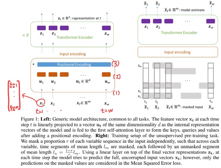
(3) Unsupervised Pre-training

“autoregressive task” of denoising the input

• idea :
  • set part of input to \(0\) & predict the masked value
• notation :
  • binary noise mask : \(\mathbf{M} \in \mathbb{R}^{w \times m}\)
  • element-wise multiplication : \(\tilde{\mathbf{X}}=\mathbf{M} \odot \mathbf{X}\)

\(\begin{gathered} \hat{\mathbf{x}}_{\mathbf{t}}=\mathbf{W}_{\mathbf{o} \mathbf{z}_{\mathbf{t}}}+\mathbf{b}_{\mathbf{o}} \\ \mathcal{L}_{\mathrm{MSE}}=\frac{1}{\mid M \mid} \sum_{(t, i) \in M} \sum_{(\hat{x}(t, i)-x(t, i))^{2}} \end{gathered}\).

• differs from original denoising autoencoders,
• in that loss only considers data from MASKED input