
Deep Adaptive Input Normalization for Time Series Forecasting (2019, 25)
Contents
- Abstract
- Introduction
- Deep Adaptive Input Normalization (DAIN)
- Adaptive Shifting layer
- Adaptive Scaling layer
- Adaptive Gating layer
0. Abstract
- DL degenerate, if data are not “properly normalized”
- data can be..
- 1) non-stationary
- 2) multimodal- nature
- propose adaptively normalizing the input TS
1. Introduction
mostly heuristically-designed normalization
to overcome…. propose DAIN (Deep Adaptive Input Normalization)
- 1) capable of “LEARNING” how data should be normalized
- 2) “ADAPTIVELY” changing the applied normalization scheme
\(\rightarrow\) effectively handle “non-stationary” & “multi-modal” data
3 sub layers
- 1) shift the data ( centering )
- 2) scaling ( standardization )
- 3) gating ( suppressing features that are irrelevant )
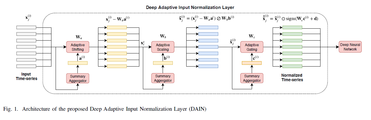
2. Deep Adaptive Input Normalization (DAIN)
Notation
- \(\left\{\mathrm{X}^{(i)} \in \mathbb{R}^{d \times L} ; i=1, \ldots, N\right\}\).
- \(\mathbf{x}_{j}^{(i)} \in \mathbb{R}^{d}, j=1,2, \ldots, L\).
- \(N\) data points (TS)
- \(L\) : length
- \(d\) : # of features
Normalization
- \(\tilde{\mathbf{x}}_{j}^{(i)}=\left(\mathbf{x}_{j}^{(i)}-\boldsymbol{\alpha}^{(i)}\right) \oslash \boldsymbol{\beta}^{(i)},\).
- ex) \(z\)-score normalization
- \(\boldsymbol{\alpha}=\left[\mu_{1}, \mu_{2}, \ldots, \mu_{d}\right]\).
- \(\boldsymbol{\beta}^{(i)}=\boldsymbol{\beta}=\left[\sigma_{1}, \sigma_{2}, \ldots, \sigma_{d}\right]\).
Propose to “dynamically estimate” these quantities
& “separately” normalize each TS, by “implicitly estimating” the distn
(1) Adaptive Shifting Layer
Shifting Operator : \(\alpha^{(i)}=\mathbf{W}_{a} \mathbf{a}^{(i)} \in \mathbb{R}^{d}\)
- summary representation : \(\mathbf{a}^{(i)}=\frac{1}{L} \sum_{j=1}^{L} \mathbf{x}_{j}^{(i)} \in \mathbb{R}^{d}\)
- \(\mathbf{W}_{a} \in \mathbb{R}^{d \times d}\) : weight matrix
Allows for exploiting possible correlations between different features
(2) Adaptive Scaling Layer
Scaling Operator : \(\boldsymbol{\beta}^{(i)}=\mathbf{W}_{b} \mathbf{b}^{(i)} \in \mathbb{R}^{d}\)
- updated summary representation : \(b_{k}^{(i)}=\sqrt{\frac{1}{L} \sum_{j=1}^{L}\left(x_{j, k}^{(i)}-\alpha_{k}^{(i)}\right)^{2}}, \quad k=1,2, \ldots, d\)
- \(\mathbf{W}_{b} \in \mathbb{R}^{d \times d}\) : weight matrix
(3) Adaptive Gating Layer
\(\tilde{\tilde{\mathbf{x}}}_{j}^{(i)}=\tilde{\mathbf{x}}_{j}^{(i)} \odot \gamma^{(i)}\).
- \(\gamma^{(i)}=\operatorname{sigm}\left(\mathbf{W}_{c} \mathbf{c}^{(i)}+\mathbf{d}\right) \in \mathbb{R}^{d}\).
- \(\mathbf{W}_{c} \in \mathbb{R}^{d \times d}\) & \(\mathrm{d} \in \mathbb{R}^{d}\) : weight
- \(\mathbf{c}^{(i)}=\frac{1}{L} \sum_{j=1}^{L} \tilde{\mathbf{x}}_{j}^{(i)} \in \mathbb{R}^{d}\).
Suppress features that are not relevant
Summary
- \(\alpha^{(i)}, \beta^{(i)}, \gamma^{(i)}\) are dependent on current ‘local’ data on window \(i\)
-
‘global’ estimates of \(\mathbf{W}_{a}, \mathbf{W}_{b}, \mathbf{W}_{c}, \mathbf{d}\) , that are trained using multiple samples on time-series, \(\left\{\mathbf{X}^{(i)} \in \mathbb{R}^{d \times L} ; i=1, \ldots, M\right\}\)
- no additional training required! (end-to-end)