(paper) A Memory Network Based Solution for MTS Forecasting

DeepHit : A Deep Learning Approach to Survival Analysis with Competing Risks

Contents

1. Abstract
2. Introduction
3. Framework
   1. Problem Formulation
   2. Memory Time-series Network

0. Abstract

RNN :

• unable to capture “extremely long-term patterns”
• lack of explainability

propose a MTNet (Memory Time-series Network)

• consists of…

  • 1) large memory component
  • 2) three separate encoders
  • 3) autoregressive components

  \(\rightarrow\) train jointly

1. Introduction

Previous Works

• Attention based encoder : remedy to vanishing gradient problem

• LSTNet : solution for MTS

  • 1) Convolutional Layer & Recurrent Layer

  • 2) Recurrent skip : capture long-term dependencies

  • 3) incorporates

    • (1) traditional autoregressive linear model
    • (2) non-linear NN

  • downside : predefined hyperparameter in Recurrent skip

    \(\rightarrow\) replace Recurrent skip with “Temporal attention layer”

• DA-RNN (Dual-stage Attention based RNN)

  • step 1) attention : extract relevant driving series
  • step 2) temporal attention : select relevant encoder hidden states across all time steps
  • downside 1) does not consider spatial correlations among different components of exogenous data
  • downside 2) point-wise attention : not suitable for capturing continuous periodical patterns

MTNet (Memory Time-series Network)

Exploit the idea of MEMORY NETWORK

propose a TSF model, that consists of..

• 1) memory component

• 2) 3 different embedding feature maps

  ( generated by 3 encoders )

• 3) autoregressive components

Calculate similarity between “input & data in memory”

\(\rightarrow\) derive “attentional weights” across all chunks of memory

Incorporate traditional autoregressive linear model

Attention :

• [DA-RNN, LSTNet] attention to particular timestamps
• [proposed] attention to period of time

2. Framework

(1) Problem Formulation

Notation

• MTS : \(\boldsymbol{Y}=\left\{\boldsymbol{y}_{1}, \boldsymbol{y}_{2}, \ldots, \boldsymbol{y}_{T}\right\}\)
  • \(\boldsymbol{y}_{t} \in \mathbb{R}^{D}\), where \(D\) : # of dimension (TS)
• predict in “ROLLING forecasting fashion”
  • input : \(\left\{\boldsymbol{y}_{1}, \boldsymbol{y}_{2}, \ldots, \boldsymbol{y}_{T}\right\}\)
  • output : \(\boldsymbol{y}_{T+h}\)

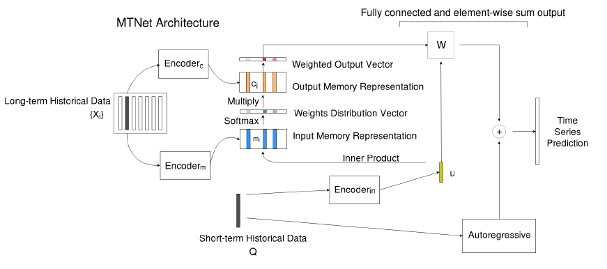
(2) Memory Time-series Network

Input :

• 1) long-term TS : \(\left\{\boldsymbol{X}_{i}\right\}=\boldsymbol{X}_{1}, \cdots, \boldsymbol{X}_{n}\)

• to be stored in memory

• 2) short-term TS : \(Q\)

  \(\rightarrow\) \(X\) & \(Q\) are not overlapped

Model

• 1) put \(\boldsymbol{X}_{i}\) inside (fixed-size) memory

• 2) embeds \(\boldsymbol{X}\) and \(Q\) into a (fixed length) representation

• with \(\text{Encoder}_m\) & \(\text{Encoder}_{in}\)

• 3) Attention : attend to blocks stored in the memory

  • inner product of their embedding

• 4) use \(\text{Encoder}_{c}\) to obtain the context vector of the memory \(X\)

  & multiply with attention weights \(\rightarrow\) get “weighted memory vectors”

• 5) concatenates …

  • (1) weighted output vectors
  • (2) embedding of \(\boldsymbol{Q}\)

  \(\rightarrow\) feed as input to a dense layer

• 6) final prediction : sum the output of

  • (1) NN
  • (2) AR model

(a) Encoder Architecture

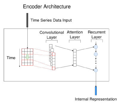
• input : \(X \in \mathbb{R}^{D \times T}\)
• use CNN w.o pooling
  • to extract (1) short-term patterns in time dimension & (2) local dependencies between variables
  • multiple kernels with
    • size \(w\) in time dimension
    • size \(D\) in variable dimension

(b) Input Memory Representation

• input : long-term historical data \(\left\{\boldsymbol{X}_{i}\right\}=\boldsymbol{X}_{1}, \cdots, \boldsymbol{X}_{n}\)
  • where \(\boldsymbol{X}_{i} \in \mathbb{R}^{D \times T}\)
• output : \(\boldsymbol{m}_{i}\) … where \(\boldsymbol{m}_{i} \in \mathbb{R}^{d}\)
  • entire set \(\left\{\boldsymbol{X}_{i}\right\}\) are converted into input memory vectors \(\left\{\boldsymbol{m}_{i}\right\}\)
• ( short-term historical data \(\boldsymbol{Q}\) is also embedded via another encoder, and get \(\boldsymbol{u}\) )

Notation

• \(\boldsymbol{m}_{i} =\operatorname{Encoder}_{m}\left(\boldsymbol{X}_{i}\right)\).
• \(\boldsymbol{u} =\operatorname{Encoder}_{i n}(\boldsymbol{Q})\).

Compute the match between..

• (1) \(\boldsymbol{u}\)
• (2) each memory vector \(\boldsymbol{m}_{i}\)

\(\rightarrow\) \(p_{i}=\operatorname{Softmax}\left(\boldsymbol{u}^{\top} \boldsymbol{m}_{i}\right)\)

(c) Output Memory Representation

context vector : \(\boldsymbol{c}_{i}=\operatorname{Encoder}_{c}\left(\boldsymbol{X}_{i}\right)\)

weighted output vector : \(\boldsymbol{o}_{i}=p_{i} \times \boldsymbol{c}_{i}\) …… where \(\boldsymbol{o}_{i} \in \mathbb{R}^{d}\)

(d) autoregressive component

\(\boldsymbol{y}_{t}^{D}=\boldsymbol{W}^{D}\left[\boldsymbol{u} ; \boldsymbol{o}_{1} ; \boldsymbol{o}_{2} ; \cdots ; \boldsymbol{o}_{T}\right]+\boldsymbol{b}\).

(e) final prediction

integrating the outputs of the (1) NN & (2) AR

• \(\hat{\boldsymbol{y}}_{t}=\boldsymbol{y}_{t}^{D}+\boldsymbol{y}_{t}^{L}\).

Loss Function : MAE

• \(\mathcal{O}\left(\boldsymbol{y}_{T}, \hat{\boldsymbol{y}}_{T}\right)=\frac{1}{N} \sum_{j=1}^{N} \sum_{i=1}^{D} \mid \left(\hat{\boldsymbol{y}}_{T, i}^{j}-\boldsymbol{y}_{T, i}^{j}\right) \mid\).