(paper) Think Globally, Act Locally ; A DNN approach to High-Dimensional TSF

Think Globally, Act Locally ; A DNN approach to High-Dimensional TSF (2019,120)

Contents

1. Abstract
2. Introduction
3. Problem Setting
4. LeveledInit : Handling Diverse Scales with TCN
5. DeepGLO : A Deep Global Local Forecaster
   1. Global : TCN-MF
   2. Combining the Global model with Local features

Abstract

HIGH-dimension TS ( millions of correlated TS)

\(\rightarrow\) need to exploit GLOBAL patterns & COUPLE them with local calibration

DeepGLO

• deep forecasting model, which thinks globally & acts locally
• hybrid model, that combines…
  • 1) global matrix factorization ( regularized by TCN )
  • 2) temporal network, that captures local properties

1. Introduction

2 shortcomings of causal convolutions

• 1) difficult to train on data, with wide variation in scales

  • ex) TS1 = [ 20,24,25,19,… ] & TS2 = [ 8000,8130,7830, …]

• 2) focus only on LOCAL past data

  • alternative : use 2D convolutions & recurrent connections

    • able to take multiple input \(\rightarrow\) capture global properties

    • but… not scale beyond thousands of TS

  • alternative ) TRMF ( Temporally Regularized Matrix Factorization )

    • express all TS as “linear combination” of basis TS
    • but…. can only model linear temporal dependencies

propose DeepGLO

• 1) think globally & act locally ( leverage both local & global patterns )
• 2) able in “wide variations” in scale

2. Problem Setting

(1) Forecasting Task

Notation

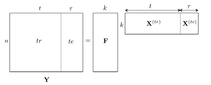
• raw TS : \(\mathbf{Y}=\left[\mathbf{Y}^{(\mathrm{tr})} \mathbf{Y}^{(\mathrm{te})}\right]\)
  • train set : \(\mathbf{Y}^{(\mathrm{tr})} \in \mathbb{R}^{n \times t}\)……. \(t\) : number of points observed
  • test set : \(\mathbf{Y}^{(\mathrm{te})} \in \mathbb{R}^{n \times \tau}\)…….. \(\tau\) : window size for forecasting
  • \(\mathbf{y}^{(i)}\) : \(i\)-th TS
• covariates : \(\mathbf{Z} \in \mathbb{R}^{n \times r \times(t+\tau)}\)
  • \(i\)-th TS and \(j\)-th time point : \(\mathbf{z}_{j}^{(i)}=\mathbf{Z}[i,:, j]\) ( \(r\)-dim )

Task :

• given original TS \(\mathbf{Y}^{(\mathrm{tr})}\) & \(\mathbf{Z}\)

• predict future in the test range ( = \(\hat{\mathbf{Y}}^{(\mathrm{te})} \in \mathbb{R}^{n \times \tau}\) )

(2) Objective

a) normalized absolute deviation ( = WAPE )

• \(\mathcal{L}\left(Y^{(\mathrm{obs})}, Y^{(\mathrm{pred})}\right)=\frac{\sum_{i=1}^{n} \sum_{j=1}^{\tau} \mid Y_{i j}^{(\mathrm{obs})}-Y_{i j}^{(\mathrm{pred})} \mid }{\sum_{i=1}^{n} \sum_{j=1}^{\tau} \mid Y_{i j}^{(\mathrm{obs})} \mid }\).

b) squared-loss

• \(\mathcal{L}_{2}\left(Y^{(\mathrm{obs})}, Y^{(\mathrm{pred})}\right)=(1 / n \tau)\left\ \mid Y^{(\mathrm{obs})}-Y^{(\mathrm{pred})}\right\ \mid _{F}^{2}\).

3. LeveledInit : Handling Diverse Scales with TCN

LeveledInit = simple initialization scheme for TCN

• designed to handle high-dim TS with wide variation in scale
• without apriori normalization

Previous works

• choice of normalization parameters have significant effect on performance

Scheme

• Goal : deal with wide variation in scale
• start with initial parameters, that results in approximately predicting the AVERAGE value of a given window of past time points \(\mathbf{y}_{j-l: j-1}\) as the future prediction \(\hat{y}_{j}\)

4. DeepGLO : A Deep Global Local Forecaster

• leverage both GLOBAL & LOCAL features
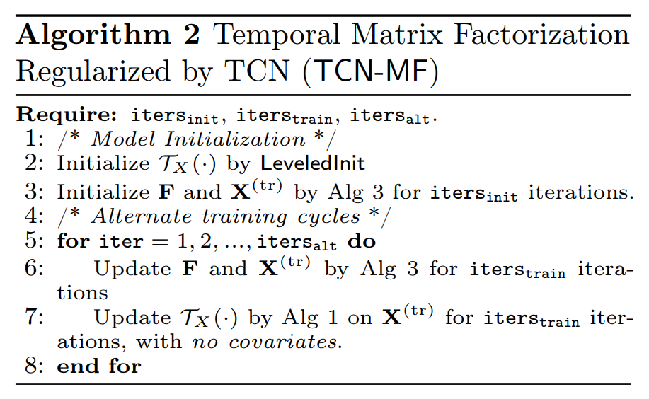
• present a global component : TCN-MF (TCN regularized Matrix Factorization)
  • represent each of TS as a linear combination of \(k\) basis TS

(1) Global : TCN-MF

propose a LOW-rank MF model

• uses TCN for regularization
• idea : factorize \(\mathbf{Y}^{(tr)}\) into low-rank factors..
  • 1) \(\mathbf{F} \in \mathbb{R}^{n \times k}\)
  • 2) \(\mathbf{X}^{(\mathrm{tr})} \in \mathbb{R}^{k \times t}\), where \(k \ll n\)
    • ( = comprised of \(k\) basis TS, that capture global temporal patterns )

Temporal Regularization by TCN

• TCN that captures temporal patterns in \(\mathbf{Y}^{(tr)}\)

  \(\rightarrow\) encourage temporal structures in \(\mathbf{X}^{(\mathrm{tr})} \in \mathbb{R}^{k \times t}\)

Regularization :

• \(\mathcal{R}\left(\mathbf{X}^{(\mathrm{tr})} \mid \mathcal{T}_{X}(\cdot)\right):=\frac{1}{ \mid \mathcal{J} \mid } \mathcal{L}_{2}\left(\mathbf{X}[:, \mathcal{J}], \mathcal{T}_{X}(\mathbf{X}[:, \mathcal{J}-1])\right)\).

Objective function :

• \(\mathcal{L}_{G}\left(\mathbf{Y}^{(\operatorname{tr})}, \mathbf{F}, \mathbf{X}^{(\operatorname{tr})}, \mathcal{T}_{X}\right):=\mathcal{L}_{2}\left(\mathbf{Y}^{(\operatorname{tr})}, \mathbf{F X}^{(\operatorname{tr})}\right)+\lambda_{\mathcal{T}} \mathcal{R}\left(\mathbf{X}^{(\operatorname{tr})} \mid \mathcal{T}_{X}(\cdot)\right)\).

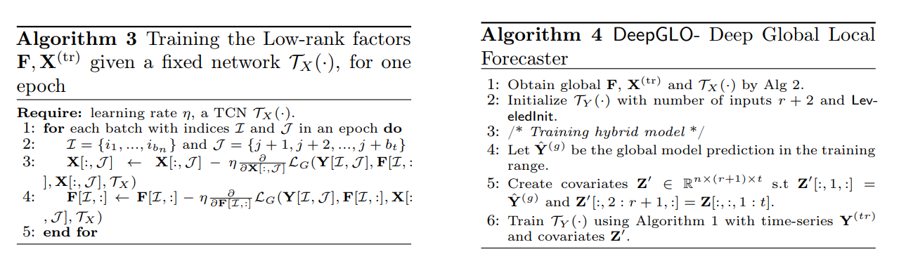
Training

low-rank factors \(\mathbf{F}\) , \(\mathbf{X}^{(tr)}\) & temporal network \(\mathcal{T}_X(\cdot)\)

\(\rightarrow\) trained alternatively, to minimize the loss!

Prediction

• trained \(\mathcal{T}_X(\cdot)\) ( local network )

  \(\rightarrow\) used for multi-step look ahead prediction

• \(\left[\hat{x}_{j-l+1}, \cdots, \hat{x}_{j}\right]:=\mathcal{T}_{X}\left(\mathbf{x}_{j-l: j-1}\right)\).

• final global predictions : \(\mathbf{Y}^{(t e)}=\mathbf{F} \hat{\mathbf{X}}^{(t e)}\)

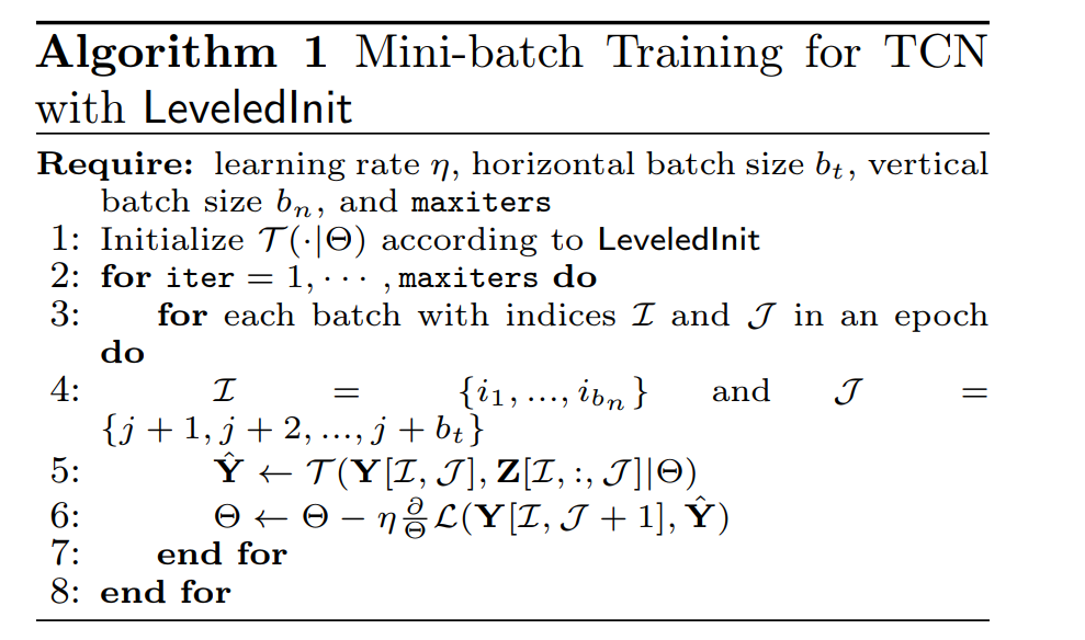
(2) Combining the Global model with Local features

Final hybrid model : TCN \(\mathcal{T}_Y(\cdot \mid \Theta_Y)\)

• input : \(\mathbf{Y}^{(\mathrm{tr})}\) & \(\mathbf{Z}\)
• predict \(\hat{\mathbf{Y}}^{(\mathrm{te})} \in \mathbb{R}^{n \times \tau}\)