(paper) COST ; Contrastive Learning of Disentangled Seasonal-Trend Representations for TS forecasting

COST ; Contrastive Learning of Disentangled Seasonal-Trend Representations for TS forecasting (2022)

Contents

1. Abstract
2. Introduction
3. Seasonal-Trend Representation for TS
4. Seasonal-Trend Contrastive Learning Framework
   1. Trend Feature Representations
   2. Seasonal Fetaure Representations

0. Abstract

promising paradigm for TS forecasting :

• (step 1) learn disentangled feature representations,
• (step 2) simple regression fine-tuning step

from a causal perspective

CoST

• propose a new TS representation learning framework

• applies contrastive learning methods, to learn disentangled seasonal-trend representations
• comprises both
  • (1) time domain contrastive losses
  • (2) frequency domain contrastive losses

1. Introduction

End-to-End (X)

• end to end ( learned representations & predictions )

  \(\rightarrow\) unable to transfer nor generalize well!

• Thus, aim to learn disentangled seasonal-trend representations

Leverage the idea of Structural TS models

• TS = T + S + error

CoST

= Contrastive Learning of Disentangled Seasonal-Trend Representations for TS forecasting

• leverages inductive biases in the model architecture
• efficiently learns Trend representations
  • mitigating the problem of lookback window selection, by introducing a mixture of auto-regressive experts
• learns powerful Seasonal representations
  • by leveraging a learnable Fourier layer
  • enables intra-frequency interactions
• domain
  • TREND : time domain
  • SEASONALITY : frequency domain

2. Seasonal-Trend Representation for TS

(1) Problem Formulation

Notation

• \(\left(\boldsymbol{x}_{1}, \ldots \boldsymbol{x}_{T}\right) \in \mathbb{R}^{T \times m}\) : MTS
• \(h\) : lookback window
• \(k\) : forecasting horizon
• \(\hat{\boldsymbol{X}}=g(\boldsymbol{X})\) : model
  • \(\boldsymbol{X} \in \mathbb{R}^{h \times m}\) : input
  • \(\hat{\boldsymbol{X}} \in \mathbb{R}^{k \times m}\) : output

Not an end-to-end model!

• instead, focus on learning feature representations from observed data
• aim to learn a nonlinear feature embedding function \(\boldsymbol{V}=f(\boldsymbol{X})\),
  • where \(\boldsymbol{X} \in \mathbb{R}^{h \times m}\) and \(\boldsymbol{V} \in \mathbb{R}^{h \times d}\),
  • map per each timestamp

Then, using the learned representations of the final timestamp \(\boldsymbol{v}_{h}\)

\(\rightarrow\) used as inputs for the downstream regressor of the forecasting task.

(2) Disentanged Seasonal-Trend Representation Learning and its Causal interpretation

Introduce structural priors for TS

• use Bayesian Structural Time Series Model

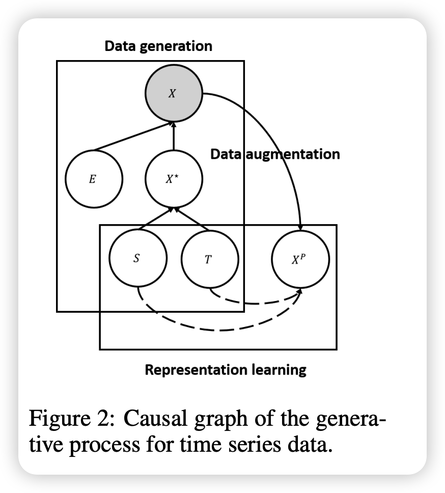
Assumption 1

• observed TS : \(X\) is generated from…
  • (1) \(E\) : error variable
  • (2) \(X^{\star}\) : error-free latent variable : generated from…
    • (2-1) \(T\) : trend variable
    • (2-2) \(S\) : seasonal variable
• Since \(E\) is not predictable…focus on \(X^{\star}\)

Assumption 2 : Independent mechanism

• season & trend do not interact with each other

  \(\rightarrow\) disentangle S & T

Learning representations for \(S\) & \(T\)

• allows us to find stable result
• since targets \(X^{\star}\) are unknown…. construct a proxy CONTRASTIVE learning task

3. Seasonal-Trend Contrastive Learning Framework

CoST framework

• learn disentangled seasonal-trend reperesentation
• for each time step, have the disentangled representations for S & T
  • \(\boldsymbol{V}=\left[\boldsymbol{V}^{(T)} ; \boldsymbol{V}^{(S)}\right] \in \mathbb{R}^{h \times d}\).
    • trend : \(\boldsymbol{V}^{(T)} \in \mathbb{R}^{h \times d_{T}}\)
    • season : \(\boldsymbol{V}^{(S)} \in \mathbb{R}^{h \times d_{S}}\)

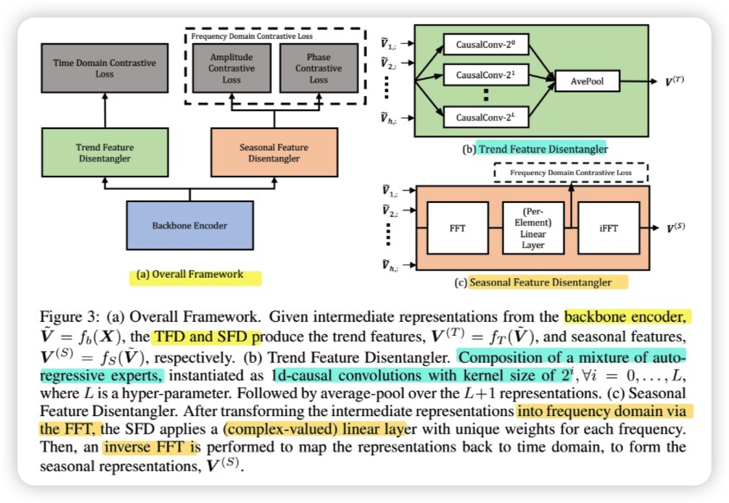
Step 1) : encoder

• encoder : \(f_{b} : \mathbb{R}^{h \times m} \rightarrow \mathbb{R}^{h \times d}\)
• map into latent space ( = intermediate representation )

Step 2) : trend & seasonal representation

• from intermediate representations..
  • (1) TFD ( Trend Feature Disentagler ) : \(f_{T}: \mathbb{R}^{h \times d} \rightarrow \mathbb{R}^{h \times d_{T}}\)
    • extracts trend representation,
    • via a mixture of AR experts
    • learned via a time domain constrastive loss \(L_{time}\)
  • (2) SFD ( Seasonal Feature Disentagler ) : \(f_{S}: \mathbb{R}^{h \times d} \rightarrow \mathbb{R}^{h \times d_{S}}\)
    • extracts seasonal representation,
    • via a learnable Fourier layer
    • learned via frequency domain constrastive loss, which consists of
      • a) \(L_{amp}\) : amplitude component
      • b) \(L_{phase}\) : phase component
• overall loss function :
  • \(\mathcal{L}=\mathcal{L}_{\text {time }}+\frac{\alpha}{2}\left(\mathcal{L}_{\mathrm{amp}}+\mathcal{L}_{\text {phase }}\right)\).
    • \(\alpha\) : trade-off between \(T\) & \(S\)

Step 3) concatenate

Concatenate the outputs of Trend and Seasonal Feature Disentaglers,

to obtain final output representations

(1) Trend Feature Representations

Autoregressive filtering

• able to capture time-lagged causal relationships from past observation

• problem : how to select lookback window?

  \(\rightarrow\) propose to use a MIXUTRE of auto-regressive exports

  ( adaptively select the appropriate lookback window )

Trend Feature Disentangler (TFD)

• mixture of \(L+1\) autoregressive experts

• implemented as 1-d causal convolution

  • input channel : \(d\)

  • output channel : \(d_T\)

  • kernel size : \(2^{i}\)

• each expert : \(\tilde{\boldsymbol{V}}^{(T, i)}=\operatorname{CausalConv}\left(\tilde{\boldsymbol{V}}, 2^{i}\right)\)

• average-pooling operation :

  • \(\boldsymbol{V}^{(T)}=\operatorname{AvePool}\left(\tilde{\boldsymbol{V}}^{(T, 0)}, \tilde{\boldsymbol{V}}^{(T, 1)}, \ldots, \tilde{\boldsymbol{V}}^{(T, L)}\right)=\frac{1}{(L+1)} \sum_{i=0}^{L} \tilde{\boldsymbol{V}}^{(T, i)}\).

Time Domain Contrastive Loss

• employ contrastive loss in time domain
• Given \(N\) Samples & \(K\) negative samples…
  • \(\mathcal{L}_{\text {time }}=\sum_{i=1}^{N}-\log \frac{\exp \left(\boldsymbol{q}_{i} \cdot \boldsymbol{k}_{i} / \tau\right)}{\exp \left(\boldsymbol{q}_{i} \cdot \boldsymbol{k}_{i} / \tau\right)+\sum_{j=1}^{K} \exp \left(\boldsymbol{q}_{i} \cdot \boldsymbol{k}_{j} / \tau\right)}\).

(2) Seasonal Fetaure Representations

spectral analysis in frequency domain

2 issues

• (1) how to support INTRA-frequency interactions

• (2) what kind of learning signal is requred to learn representations,

  which are able to discriminate between different seasonality patterns

\(\rightarrow\) introduce SFD, which makes use of a learnable Fourier Layer

​ ( SFD = Seasonal Feature Disentangler )

Seasonal Feature Disentangler (SFD)

composed of 2 parts

• (1) DFT (discrete Fourier Transform)
  • map intermediate features to FREQUENCY domain ( \(\mathcal{F}(\tilde{\boldsymbol{V}}) \in \mathbb{C}^{F \times d}\) )
• (2) learnable Fourier layer
  • map in to \(\boldsymbol{V}^{(S)} \in \mathbb{R}^{h \times d_{S}}\)

Model

• \(V_{i, k}^{(S)}=\mathcal{F}^{-1}\left(\sum_{j=1}^{d} A_{i, j, k} \mathcal{F}(\tilde{\boldsymbol{V}})_{i, j}+B_{i, k}\right)\).

Frequency Domain Contrastive Loss

discriminate between different periodic patterns, given an frequency

• \(\mathcal{L}_{\mathrm{amp}}=\frac{1}{F N} \sum_{i=0}^{F} \sum_{j=1}^{N}-\log \frac{\exp \left( \mid \boldsymbol{F}_{i,:}^{(j)} \mid \cdot \mid \left(\boldsymbol{F}_{i,:}^{(j)}\right)^{\prime} \mid \right)}{\exp \left( \mid \boldsymbol{F}_{i,:}^{(j)} \mid \cdot \mid \left(\boldsymbol{F}_{i,:}^{(j)}\right)^{\prime} \mid \right)+\sum_{k \neq j}^{N} \exp \left( \mid \boldsymbol{F}_{i,:}^{(j)} \mid \cdot \mid \boldsymbol{F}_{i,:}^{(k)} \mid \right)}\).
• \(\mathcal{L}_{\text {phase }}=\frac{1}{F N} \sum_{i=0}^{F} \sum_{j=1}^{N}-\log \frac{\exp \left(\phi\left(\boldsymbol{F}_{i,:}^{(j)}\right) \cdot \phi\left(\left(\boldsymbol{F}_{i,:}^{(j)}\right)^{\prime}\right)\right)}{\exp \left(\phi\left(\boldsymbol{F}_{i,:}^{(j)}\right) \cdot \phi\left(\left(\boldsymbol{F}_{i,:}^{(j)}\right)^{\prime}\right)\right)+\sum_{k \neq j}^{N} \exp \left(\phi\left(\boldsymbol{F}_{i,:}^{(j)}\right) \cdot \phi\left(\boldsymbol{F}_{i,:}^{(k)}\right)\right)}\).

where \(\boldsymbol{F}_{i,:}^{(j)}\) is the \(j\)-th sample in a mini-batch, and \(\left(\boldsymbol{F}_{i,:}^{(j)}\right)^{\prime}\) is the augmented version of that sample.