(paper) SSDNet ; State Space Decomposition NN for TS Forecasting

SSDNet : State Space Decomposition NN for TS Forecasting (2021)

Contents

1. Abstract
2. Problem Formulation
3. SSDNet
   1. Network Architecture
   2. Loss Function

0. Abstract

SSDNet = (1) Transformer + (2) SSM

• probabilistic & interpretable forecasts

  ( including trend & seasonality components )

Use of Transformer

• to learn temporal patterns
• to estimate the parameters of SSM directly

1. Problem Formulation

3 tasks

• (1) solar power forecasting
• (2) electricity demand forecasting
• (3) exchange rate forecasting

Input (Notation)

• (1) \(N\) univariate TS : \(\left\{\mathbf{Y}_{i, 1: T_{l}}\right\}_{i=1}^{N}\)
  • \(\mathbf{Y}_{i, 1: T_{l}}:=\left[y_{i, 1}, y_{i, 2}, \ldots, y_{i, T_{l}}\right]\).
  • \(y_{i, t} \in \Re\) : value of \(i\)-th TS at time \(t\)
• (2) multi-dim covariates : \(\left\{\mathbf{X}_{i, 1: T_{l}+T_{h}}\right\}_{i=1}^{N}\)

Goal

• predict \(\left\{\mathbf{Y}_{i, T_{l}+1: T_{l}+T_{h}}\right\}_{i=1}^{N}\)

SSDNet

produces a pdf of future values :

\(p\left(\mathbf{Y}_{i, T_{l}+1: T_{l}+T_{h}} \mid \mathbf{Y}_{i, 1: T_{l}}, \mathbf{X}_{i, 1: T_{l}+T_{h}} ; \Phi\right) =\prod_{t=T_{l}+1}^{T_{l}+T_{h}} p\left(y_{i, t} \mid \mathbf{Y}_{i, 1: t-1}, \mathbf{X}_{i, 1: t} ; \Phi\right)\),

2. SSDNet

2-1. Network Architecture

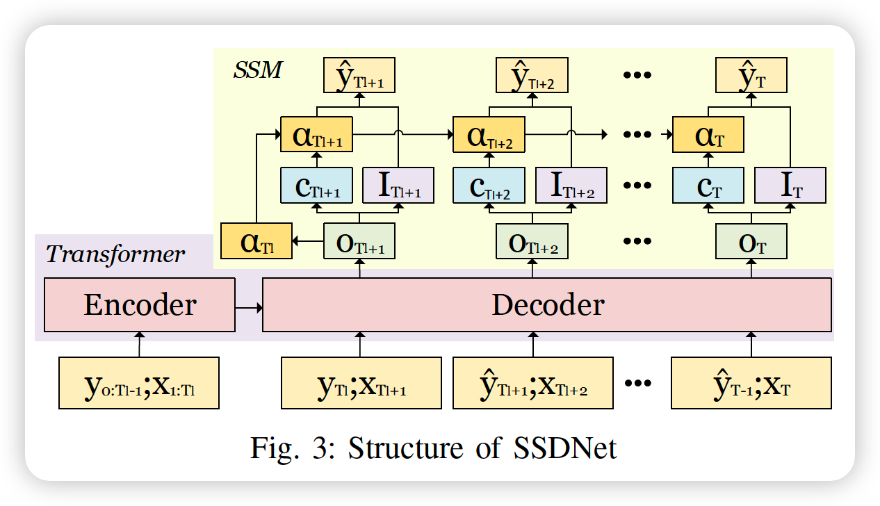
a) SSDNet

• (1) Transformer + (2) SSM
• 2 feed forward steps

b) traditional SSM vs SSDNet

• SSDNet : remove random noise part

• SSM (of SSDNet) does not process historical series directly,

  rather, uses latent component generated by Transformer

c) Steps

[ Step 1 ]

• Transformer generates latent components
• this latent component is used to estimate SSM params & variance of forecast

[ Step 2 ]

• SSM takes the state vector from the previous step
• uses it to predict mean of forecast

d) Details

• step 1) Transformer extracts latent components \(o_{t}\),

  • from time series \(y_{1: T_{l}}, x_{1: T_{t}}\)

  • \(o_{t}=f\left(y_{1: T_{l}}, x_{1: T_{t}}\right)\).

• step 2) employ additive TS decomoposition model

  • in the form of SSM
  • \(\hat{y}_{t}\) = \(T_{t}\) + \(S_t\) + \(I_t\) ( = probability component )
  • step 2) in detail :
    • \(\hat{y}_{t}=z_{t}^{T} \alpha_{t}+I_{t}, \quad t=1, \ldots, T_{h}\).
      • \(\alpha_{t+1}=\Gamma_{t} \alpha_{t}+c_{t}\).
      • \(I_{t} \sim \mathcal{N}\left(0, \sigma_{I_{t}}^{2}\right)\).
    • \(\alpha_{t} \in \Re^{s \times 1}\) : latent state vector
      • it contains trend ( \(\operatorname{Tr}_{t}\) ) & seasonality ( \(S_{t}\))
      • \(s\) : number of seasonality
    • \(c_{t} \in \Re^{s \times 1}\) : innovation term
      • allow SSDNet to learn stochastic trends with fluctuations in TS

e) etc

Innovation term ( \(c_t\) ) & Variance ( \(o^2_{I_t}\) )

• learnt from latent factor \(o_t\)
• \(\begin{aligned} \sigma_{I_{t}}^{2}=g_{s}\left(o_{t}\right) &=\operatorname{Softplus}\left(\operatorname{Linear}\left(o_{t}\right)\right) \\ &=\log \left(1+\exp \left(\operatorname{Linear}\left(o_{t}\right)\right)\right) \\ \end{aligned}\).
• \(\begin{aligned} c_{t}=g_{c}\left(o_{t}\right)=& \operatorname{HardSigmoid}\left(\operatorname{Linear}\left(o_{t}\right)\right)-0.5 \\ &= \begin{cases}-0.5 & \text { if } \mathrm{x} \leq-3 \\ 0.5 & \text { if } \mathrm{x} \geq+3 \\ \text { Linear }\left(\mathrm{o}_{\mathrm{t}}\right) / 6 & \text { otherwise }\end{cases} \end{aligned}\).

\(\Gamma_{t}\) and \(z_{t}\) are non-trainable and fixed for all time steps

\(\alpha_{t}=\left(\begin{array}{c} \operatorname{Tr}_{t} \\ S_{1: s-1, t} \end{array}\right), z_{t}=\left(\begin{array}{l} 1 \\ 1 \\ 0_{s-2} \end{array}\right)\).

\(\Gamma_{t}=\left(\begin{array}{ccc} 1 & 0_{s-2}^{\prime} & 0 \\ 0 & -1_{s-2}^{\prime} & -1 \\ 0_{s-2} & I_{s-2} & 0_{s-2} \end{array}\right)\).

Initial values

• \(\alpha_{0}=g_{c}\left(o_{T_{l+1}}\right)=\operatorname{HardSigmoid}\left(\operatorname{Linear}\left(o_{T_{l+1}}\right)\right)-0.5\).

f) summary

\(\hat{y}_{t} \sim \mathcal{N}\left(T r_{t}+S_{t}, \sigma_{I_{t}}^{2}\right)\).

• predictions are sampled from the distribution
• \(\rho\)-quantile output could be generated via the inverse CDF

2-2. Loss Function

• For accurate point & probabilistic forecasts

• combine MAE & NLL