(paper) Change Point Detection in Time Series Data using Autoencoders with a Time-Invariant Representation

Change Point Detection in Time Series Data using Autoencoders with a Time-Invariant Representation (2020, 4)

Contents

1. Abstract
2. Introduction
3. Problem Formulation
4. AE based CPD
   1. Preprocessing
   2. Feature Encoding
   3. Post processing & Peak detection

0. Abstract

CPD = locate abrupt property changes

This paper…

• uses autoencoder (AE) based methodology with novel loss function

• mitigate the issue of false detection alarms using a post-processing procedure

Allow user to indicate whether

• change points should be sought in time domain, frequency domain, or both

Detectable change points : abrupt changes in…

• slope / mean / variance / autocorrelation / frequency spectrum

1. Introduction

CPD’s goal

• 1) goal in itself
• 2) pre-processing tool to segment a TS in homogeneous segments

CPD’s categories

• 1) online CPD :

  • real-time detection
  • dissimilarity = based on difference in distn of 2 intervals

• 2) retrospective (offline) CPD :

  • robust detections

  • at the cost of needing more future data

  • ( this paper focuses on this method )

Many CPD algorithms compare “past & future TS”, by means of “dissimilarity” measure

Past Works ( algorithm : assumption(model) )

• ex 1) CUSUM : parametric probability distribution
• ex 2) GLR : autoregressive model
• ex 3) subspace method : state-space model
• ex 4) Bayesian online CPD

\(\rightarrow\) performance depends on “how well actual data follows the assumed model”

• ex 5) KDE : parameter free
• ex 6) Related Density Ratio estimation : parameter free

ex 7) autoencoder

• pros

  • absence of distn assumptions
  • extract complex features in cost-efficient ways

• cons

  • no guarantee that distance between consecutive features reflect actual dissimilarity

  • correlated nature of TS samples is not properly used
  • absence of post-processing procedure preceding detection of peaks in the dissimilarity measure leads to high FP detection alarms

TIRE (partially Time Invariate REpresentation)

• new AE-based CPD

• contribution

  • 1) novel adaptation of AE with a loss function that promotes time-invariant features ( + define new dissimilarity measure )

  • 2) focus on non-iid data, use discrete Fourier transform to obtain temporally localized spectral information, propose an approach that combines “time & frequency” domain info

2. Problem Formulation

\(\mathbf{X}\) : time series of…

• # of channel : \(d\)
  • \(\mathbf{X}^{i}\) : \(i\)th channel
• length : \(T\) ( where \(0=T_{0} < T_1 < \cdots < T_p = T\) )
  • \(T_1, T_2, \cdots\) : change points

\(\left(\mathbf{X}\left[T_{k}+1\right], \ldots, \mathbf{X}\left[T_{k+1}\right]\right)\) : subsequence of time series

• realization of discrete time weak-sense stationary stochastic (WSS) process

Goal of CPD

• estimate change points, w.o prior knowledge on “number & location”

Dissimilarity Measure

• dissimilarity between (a) & (b)
  • (a) \((\mathbf{X}[t-N+1], \ldots, \mathbf{X}[t])\)
  • (b) \((\mathbf{X}[t+1], \ldots, \mathbf{X}[t+N])\)
• \(N\) : user defined “window size”

Goal (1) :

• develop a CPD-tailored feature embedding
• and corresponding dissimilarity measure \(D_t\)
  • ( \(D_t\) peaks, when the WSS restriction is violated )

Goal (2) :

• determine all local maxima
• label each local maximum, which exceed certain threshold \(\tau\)

3. AE based CPD

(1) Preprocessing

step 1) divide each channel into window size of \(N\)

• \(\mathbf{x}_{t}^{i}=\left[\mathbf{X}^{i}[t-N+1], \ldots, \mathbf{X}^{i}[t]\right]^{T} \in \mathbb{R}^{N}\).

step 2) combine for every \(t\) ( into single vector )

• \(\mathbf{y}_{t}=\left[\left(\mathbf{x}_{t}^{1}\right)^{T}, \ldots,\left(\mathbf{x}_{t}^{d}\right)^{T}\right]^{T} \in \mathbb{R}^{N d}\).

step 3) Transformation

• (1) : DFT (discrete Fourier transform)
  • DFT on each window
    • to obtain “temporally localized spectral information”

• (2) : cropped to length \(M\)

• (1) + (2) = \(\mathcal{F}: \mathbb{R}^{N} \rightarrow \mathbb{R}^{M}\)

• \(\mathbf{z}_{t}=\left[\mathcal{F}\left(\mathbf{x}_{t}^{1}\right)^{T}, \ldots, \mathcal{F}\left(\mathbf{x}_{t}^{d}\right)^{T}\right]^{T} \in \mathbb{R}^{M d}\)>

  ( = frequency-domain counterpart of \(y_t\) )

(2) Feature Encoding

[1] use AEs to extract features…

• from **time-domain(TD) windows **\(\left\{\mathbf{y}_{t}\right\}_{t}\)

• from frequency-domain (FD) windows \(\left\{\mathbf{z}_{t}\right\}_{t}\).

[2] proposal of new loss function

• that promotes time-invariance of the features in consecutive windows

Notation

• ENC input : \(\mathbf{y}_{t} \in \mathbb{R}^{N d}\)
• ENC output : \(\mathbf{h}_{t}=\sigma\left(\mathbf{W} \mathbf{y}_{t}+\mathbf{b}\right)\)
• DEC output : \(\tilde{\mathbf{y}}_{t}=\sigma^{\prime}\left(\mathbf{W}^{\prime} \mathbf{h}_{t}+\mathbf{b}^{\prime}\right)\)
  • choose \(\sigma=\sigma^{\prime}\) to be the hyperbolic tangent function
• minimize \(\mid \mid \mathbf{y}_{t} - \tilde{\mathbf{y}}_{t} \mid \mid\)

BUT, \(\mathbf{h}_t\) will also contain information “NOT relevant to CPD”

• ex) phase shift, noise …

\(\rightarrow\) solve by introducing….

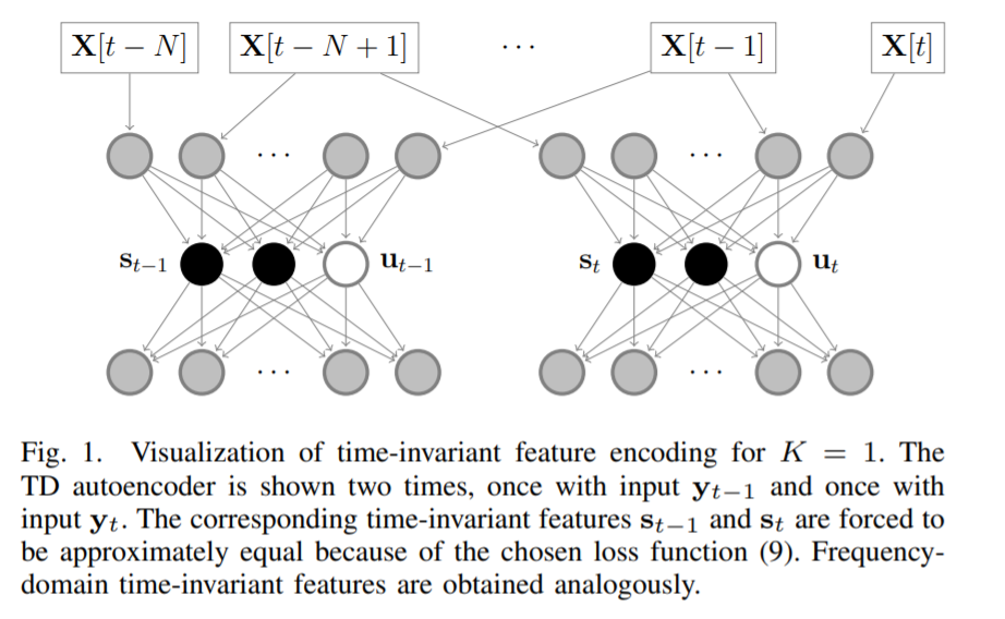
\(\mathbf{h}_{t}=\left[\left(\mathbf{s}_{t}\right)^{T},\left(\mathbf{u}_{t}\right)^{T}\right]^{T}\).

• 1) time invariant features : \(\mathbf{s}_{t} \in \mathbb{R}^{s}\)
  • invariant over time within a WSS segment
  • ex) mean, amplitude, frequency
• 2) instantaneous features : \(\mathbf{u}_{t} \in \mathbb{R}^{h-s}\)
  • all other info

Minimize the loss function…

• (original) \(\sum_{t}\left( \mid \mid \mathbf{y}_{t}-\tilde{\mathbf{y}}_{t} \mid \mid _{2}+\lambda \mid \mid \mathbf{s}_{t}-\mathbf{s}_{t-1} \mid \mid _{2}\right)\)

• (SGD) \(\sum_{t \in \mathcal{T}_{j}}\left( \mid \mid \mathbf{y}_{t}-\tilde{\mathbf{y}}_{t} \mid \mid _{2}+\lambda \mid \mid \mathbf{s}_{t}-\mathbf{s}_{t-1} \mid \mid _{2}\right)\)

• but, \(t \in \mathcal{T}_{j}\) does not generally imply that \(t-1 \in \mathcal{T}_{j}\).

  \(\rightarrow\) \(\sum_{t \in \mathcal{T}_{j}}\left( \mid \mid \mathbf{y}_{t}-\tilde{\mathbf{y}}_{t} \mid \mid _{2}+\frac{\lambda}{K} \sum_{k=0}^{K-1} \mid \mid \mathbf{s}_{t-k}-\mathbf{s}_{t-k-1} \mid \mid _{2}\right)\).

  • can think of it as \(K+1\) parallel autoencoders

the number of instantaneous features should be taken as small as possible!

(3) Post processing & Peak detection

construct dissimilarity measure!

1) Postprocessing

• combine TD & FD time-invariant features into single feature!
• \(\mathbf{s}_{t}=\left[\alpha \cdot\left(\mathbf{s}_{t}^{\mathrm{TD}}\right)^{T}, \beta \cdot\left(\mathbf{s}_{t}^{\mathrm{FD}}\right)^{T}\right]^{T}\).
  • zero-delay weighted moving average filter to smoothen!
  • \(\tilde{\mathbf{s}}_{t}[i]=\sum_{k=-N+1}^{N-1} \mathbf{v}[N-k] \cdot \mathbf{s}_{t+k}[i]\).
    • triangular shaped weighting window

Dissimilarity measure

• \(\mathcal{D}_{t}= \mid \mid \tilde{\mathbf{s}}_{t}-\tilde{\mathbf{s}}_{t+N} \mid \mid _{2}\).
• by expert knowledge…
  • case 1) \(\alpha=1\) and \(\beta=0\)
  • case 2) \(\alpha=0\) and \(\beta=1\)
  • case 3) \(\alpha=Q\left(\left\{\mathcal{D}_{t}^{\mathrm{FD}}\right\}_{t}, 0.95\right) \quad \text { and } \quad \beta=Q\left(\left\{\mathcal{D}_{t}^{\mathrm{TD}}\right\}_{t}, 0.95\right)\).

2) Peak Detection

difficult to automatically select a representative peak!

\(\rightarrow\) propose to reuse the impulse response \(\mathbf{v}\) from the moving average filtering

\(\tilde{\mathcal{D}}_{t}=\sum_{k=-N+1}^{N-1} \mathbf{v}[N-k] \cdot \mathcal{D}_{t+k} .\).

detected alarms correspond to all local maxima of \(\left(\tilde{\mathcal{D}}_{N}, \tilde{\mathcal{D}}_{N+1}, \ldots, \tilde{\mathcal{D}}_{T-N}\right)\).

Prominence of peak : minimum height needed

Given that \(\mathcal{D}_t\) is a local maximum…

• step 1) define the 2 closest time stamps left & right of \(t\), for which the dissimilarity measure is larger than \(\mathcal{D}_t\) ( = \(t_L\) & \(t_R\) )
  • \(t_{L} =\max \left\{\sup \left\{t^{*} \mid \mathcal{D}_{t^{*}}>\mathcal{D}_{t} \text { and } t^{*}<t\right\}, N\right\}\).
  • \(t_{R} =\min \left\{\inf \left\{t^{*} \mid \mathcal{D}_{t^{*}}>\mathcal{D}_{t} \text { and } t^{*}>t\right\}, T-N\right\}\).
• step 2) Prominence \(\mathcal{P}(\mathcal{D}_t)\) of local maximum \(\mathcal{D}_t\) :
  • \(\mathcal{P}\left(\mathcal{D}_{t}\right)=\mathcal{D}_{t}-\max \left\{\min _{t_{L}<t^{*}<t} \mathcal{D}_{t^{*}}, \min _{t<t^{*}<t_{R}} \mathcal{D}_{t^{*}}\right\}\).