(paper) Recurrent Neural Networks for MTS with Missing Values

Recurrent Neural Networks for MTS with Missing Values (2018, 1114)

Contents

1. Abstract
2. Introduction
3. Methods
   1. Notations
   2. GRU-RNN for TSC
   3. GRU-D : model with trainable decays

0. Abstract

• data : MTS with missing values

• missing patterns are correlated with “target labels”

• propose GRU-D

  • based on GRU

  • takes 2 representations of missing patterns

    • 1) masking
    • 2) time interval

  • not only captures “LONG-term temporal dependencies”

    but also utilizes the “MISSING PATTERNS”

1. Introduction

Missing Values are often “Informative Missingness”

\(\rightarrow\) missing values & patterns provide rich information about target labels

( = often correlated with labels )

Various approaches to deal with missing values

• 1) omission
• 2) data imputation
  • do not capture variable correlation & complex patterns
  • ex) spectral analysis, kernel methods, EM algorithm, matrix completion/factirization
• 3) multiple imputation
  • (data imputation x n) & average them

After imputation, build model! \(\rightarrow\) 2 step process ( not effective )

RNN based models

• RNNs for missing data have been studied
• ex) concatenate missing entries/timestamps with the **input **
• but no works related to “TSC”

GRU-D

• propose novel DL method

• 2 representations of informative missingness patterns

  • 1) masking :
    • informs the model “which inputs are observed”
  • 2) time interval
    • encapsulates the input observation patterns

• not only captures “LONG-term temporal dependencies”

  but also utilizes the “MISSING PATTERNS”

2. Methods

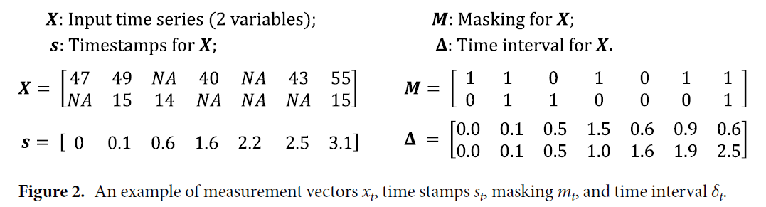
(1) Notations

\(X=\left(x_{1}, x_{2}, \ldots, x_{T}\right)^{T} \in \mathbb{R}^{T \times D}\).

• \(t \in\{1,2, \ldots, T\}, x_{t} \in \mathbb{R}^{D}\).

• \(x_{t}^{d}\) : \(d\)-th variable of \(x_t\)

• \(D\): # of variables
• \(T\) : length

\(s_{t} \in \mathbb{R}\) : time stamp when the \(t\)-th observation is obtained

• assume first observation is made at time stamp 0 ( \(s_{1}=0\) )

\(m_{t} \in\{0,1\}^{D}\) : masking vector

• denote which variables are missing
• \(m_{t}^{d}= \begin{cases}1, & \text { if } x_{t}^{d} \text { is observed } \\ 0, & \text { otherwise }\end{cases}\).

Time interval ( since its last observation )

\(\delta_{t}^{d}= \begin{cases}s_{t}-s_{t-1}+\delta_{t-1}^{d}, & t>1, m_{t-1}^{d}=0 \\ s_{t}-s_{t-1}, & t>1, m_{t-1}^{d}=1 \\ 0, & t=1\end{cases}\).

Goal : Time Series Classification

• predict labels \(l_{n} \in\{1, \ldots, L\}\)
• given…
  • 1) \(\mathcal{D}=\left\{\left(X_{n}, s_{n}, M_{n}\right)\right\}_{n=1}^{N}\).
  • 2) \(X_{n}=\left[x_{1}^{(n)}, \ldots, x_{T_{n}}^{(n)}\right]\).
  • 3) \(s_{n}=\left[s_{1}^{(n)}, \ldots, s_{T_{n}}^{(n)}\right]\).
  • 4) \(M_{n}=\left[m_{1}^{(n)}, \ldots, m_{T_{n}}^{(n)}\right]\).

(2) GRU-RNN for TSC

output of GRU at the last step \(\rightarrow\) predict labels

3 ways to handle missing values (w.o imputation)

• 1) GRU-Mean

  replace each missing observation with “mean of the variable”

  • \(x_{t}^{d} \leftarrow m_{t}^{d} x_{t}^{d}+\left(1-m_{t}^{d}\right) \widetilde{x}^{d}\).
    • where \(\tilde{x}^{d}=\sum_{n=1}^{N} \sum_{t=1}^{T_{n}} m_{t, n}^{d} x_{t, n}^{d} / \sum_{n=1}^{N} \sum_{t=1}^{T_{n}} m_{t, n}^{d}\).
    • \(\widetilde{x}^{d}\) is calculated only by “training dataset”

• 2) GRU-Forward

  replace it with last measurement

  • \(x_{t}^{d} \leftarrow m_{t}^{d} x_{t}^{d}+\left(1-m_{t}^{d}\right) x_{t^{\prime}}^{d}\).
    • where \(t^{\prime}<t\) is the last time the \(d\)-th variable was observed

• 3) GRU-Simple

  just indicate “which variables are missing” & “how long they have been missing”

  • \(x_{t}^{(n)} \leftarrow\left[x_{t}^{(n)} ; m_{t}^{(n)} ; \delta_{t}^{(n)}\right]\).

Problems

• 1), 2) …. cannot distinguish whether missing values are imputed/observed
• 3) … fails to exploit the temporal structure of missing values

(3) GRU-D : model with trainable decays

Characteristic of health-care data

• 1) missing variables tend to be close to some default value,

  if its last observation happens long time ago

• 2) influence of the input fades away over time

\(\rightarrow\) propose GRU-D to capture both!

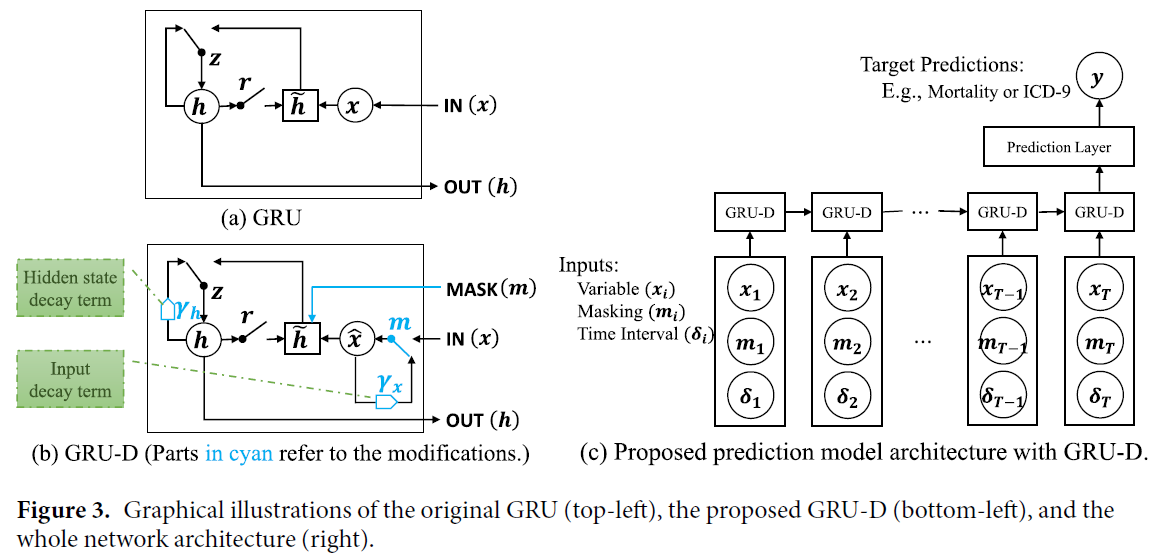
Introduce “decay rates (\(\gamma\))”,

• \(\gamma_{t}=\exp \left\{-\max \left(0, W_{\gamma} \delta_{t}+b_{\gamma}\right)\right\}\).

to control decay mechanism, by considering…

• 1) decay rates should differ from variable
• 2) “learn” decay rates

Incorporates 2 different “trainable decay” mechanism

• 1) input decay \(\gamma_{x}\)
• 2) hidden state decay \(\gamma_{h}\)

Input decay

\(\hat{x}_{t}^{d}=m_{t}^{d} x_{t}^{d}+\left(1-m_{t}^{d}\right)\left(\gamma_{x_{t}}^{d} x_{t^{\prime}}^{d}+\left(1-\gamma_{x_{t}}^{d}\right) \widetilde{x}^{d}\right)\).

• \(x_{t^{\prime}}^{d}\) : last observation of \(d\)-th variable
• \(\tilde{x}^{d}\) : empirical mean of \(d\)-th variable
• constrain \(W_{\gamma_{x}}\) to be diagonal
  • decay rate of each input variable to be “independent”

Hidden state decay

\(\hat{h}_{t-1}=\gamma_{h_{t}} \odot h_{t-1}\).

• to capture “richer knowledge” from missingness!
• do not constrain \(W_{\gamma_h}\)

Comparison

1) \(x_{t}\) and \(h_{t-1}\) \(\rightarrow\) \(\hat{x}_{t}\) and \(\hat{h}_{t-1}\)

2) masking vector \(m_{t}\) are fed into model

• \(V_{r}, V_{r}, V\) are new parameters