CNN Architectures For Large-scale Audio Classification (ICASSP 2017)
https://ieeexplore.ieee.org/stamp/stamp.jsp?tp=&arnumber=7952132&tag=1
Contents
- Abstract
- Introduction
- Dataset
- Experimental Framework
- Training
- Evaluation
- Experiments
Abstract
CNN architectures to classify the soundtracks of a dataset of \(70 \mathrm{M}\) training videos ( 5.24 million hours) with 30,871 video-level labels.
- DNNs
- AlexNet
- VGG INception
- ResNet
Experimenets on Audio Set Acoustic Event Detection (AED) classification task
1. Introduction
YouTube-100M dataset to investigate
- Q1) How popular DNNs compare on video soundtrack classification
- Q2) How performance varies with different training set and label vocabulary sizes
- Q3) Whether our trained models can also be useful for AED
Conventional methods
Conventional AED
-
Features : MFCCs
-
Classifiers : GMMs, HMMs, NMF, or SVMs
( recently; CNNs, RNNs )
Conventional datasets
-
TRECVid [14], ActivityNet [15], Sports1M [16], and TUT/DCASE Acoustic scenes 2016 [17]
\(\rightarrow\) much smaller than YouTube-100M.
RNNs and CNNs have been used in Large Vocabulary Continuous Speech Recognition (LVCSR)
\(\rightarrow\) Labels apply to entire videos without any changes in time
2. Dataset
YouTube-100M data set += 100 million YouTube
- 70M training videos
- 20M validation videos
- 10M evaluation videos
Each video:
- avg) 4.6 minute \(\rightarrow\) total 5.4M hourrs
- avg) 5 labels
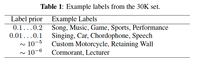
- labeled with 1 or more topic identifies ( among 30871 labels )
- labels are assigned automatically based on a combination of metadata
Videos average 4.6 minute each for a total of 5.4M training hours
3. Experimental Framework
(1) Training
Framing
Audio : divided into non-overlapping 960 ms frames
\(\rightarrow\) 20 billion examples (frames) from the 70M videos
( inherits all the labels of its parent video 0
Preprocessing to frames
Each frame is …
-
decomposed with a STFT applying 25ms windows evey 10 ms
-
resulting spectrogram is integrated into 64 mel-spaced frequency bins
-
magnitude of each bin is log-transformed
( + after adding a small offset to avoid numerical issues )
\(\rightarrow\) RESULT: log-mel spectrogram patches of 96 \(\times\) 64 bins ( = INPUT to cls )
Other details
-
batch size = 128 (randomly from ALL patches)
-
BN after all CNN layers
-
final: sigmoid layer ( \(\because\) multi-LAYER classification )
-
NO dropout, NO weight decay, NO regularization …
( no overfitting due to 7M dataset )
-
During training, we monitored progress via 1-best accuracy and mean Average Precision (mAP) over a validation subset.
(2) Evaluation
10M evaluation videos
\(\rightarrow\) create 3 balanced evaluation sets ( 33 examples per class )
- set 1) 1M videos ( 30K labels )
- set 2) 100K videos ( 3K labels )
- set 3) 12K videos ( for 400 most frequent labels )
Metric
- (1) balanced average across all classes of AUC
- (2) mean Average Precision (mAP)
3. Experiments
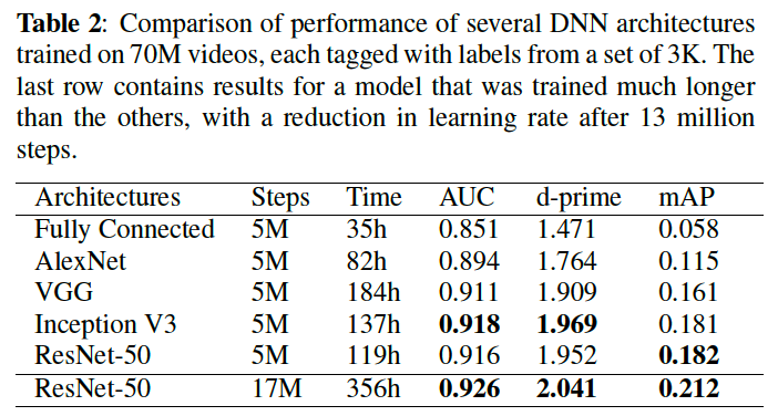
(1) Arhictecture comparison
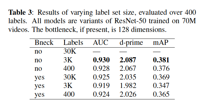
(2) Label Set Size
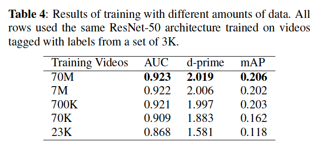
(3) Training Set Size
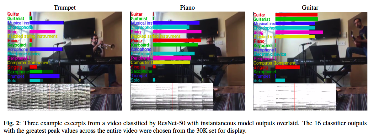
(4) Qualitative Result