Speaker Recognition from Raw Waveform with SincNet ( IEEE Spoken Language Technology Workshop 2018 )
https://arxiv.org/pdf/1808.00158.pdf
https://seunghan96.github.io/mult/ts/audio/study-(multi)Neural-Feature-Extraction-of-signal-data2/
Contents
- Abstract
- Introduction
- SincNet
- Standard CNN
- CNN in SincNet
- Hamming window
- Experiments
- Corpora
- Setup
- Baseline setup
- Result
- Filter Analysis
- Speaker Identification
- Speaker Verification
Abstract
Speaker recognition
- promising result with CNNs
( when fed by raw speech samples directly, instead of hand-crafted features )
-
latter CNNs learn low-level speech representations from waveforms
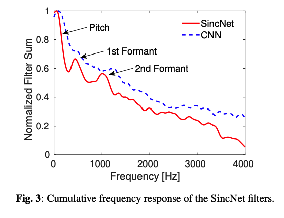
\(\rightarrow\) allowing the network to better capture important narrow-band speaker characteristics
( ex. pitch, formants )
SincNet
- novel CNN architecture
- encourages the FIRST convolutional layer to discover more meaningful filters
- parametrized sinc functions ( = band-pass filters )
-
Standard CNN vs. SincNet
- standard) learn all elements of each filter
- SincNet) only low and high cutoff frequencies are directly learned from data
\(\rightarrow\) very compact and efficient way to derive a customized filter bank
Experiments
- speaker identification task
- speaker verification task
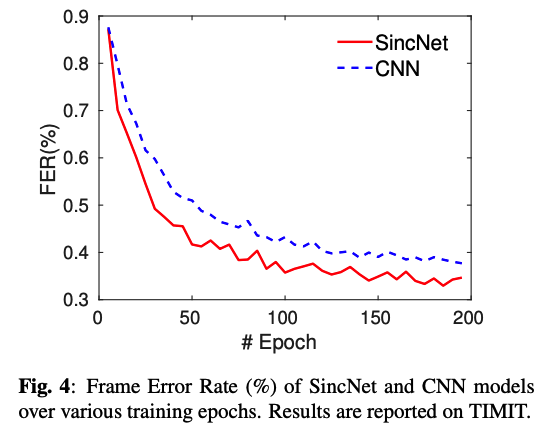
\(\rightarrow\) SincNet converges faster and performs better than a standard CNN on raw waveforms
1. Introduction
Speaker recognition
- SOTA: based on the i-vector representation of speech segments
- significant improvements over previous Gaussian Mixture Model-Universal Background Models (GMMUBMs)
- Deep learning has shown remarkable success
DNNs vs. Past works
[ DNNs ]
- have been used within the i-vector framework
- to compute Baum-Welch statistics, or for frame-level feature extraction
- have also been proposed for direct discriminative speaker classification
**[ Past works] **
-
employed hand-crafted features
ex) FBANK and MFCC coefficients
- originally designed from perceptual evidence and there are no guarantees that such representations are optimal for all speech-related tasks
- ex) Standard features
- smooth the speech spectrum, possibly hindering the extraction of crucial narrow-band speaker characteristics such as pitch and formants.
CNNs
-
most popular architecture for processing raw speech samples
-
characteristics
- weight sharing
- local filters
- pooling
\(\rightarrow\) help discover robust and invariant representations.
This paper :
The most critical part of current waveform-based CNNs is the first convolutional layer
- deals with high-dimensional inputs
- more affected by vanishing gradient problems ( when DEEP layers )
Proposes to add some constraints on the first CNN layer
-
Standard CNN : filterbank characteristics depend on several parameters
- (each element of the filter vector is directly learned)
-
SincNet : convolves the waveform with a set of parametrized sinc functions that implement band-pass filters.
-
The low and high cutoff frequencies are the only parameters of the filter learned from data.
\(\rightarrow\) still offers considerable flexibility, but forces the network to focus on high-level tunable parameters with broad impact on the shape and bandwidth of the resulting filter.
-
Results achieved on a variety of datasets
- (1) converges faster and achieves better end task performance than a more standard CNN
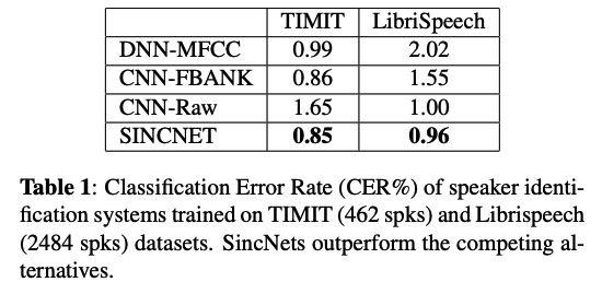
- (2) outperforms a more traditional speaker recognition system based on i-vectors
2. SincNet
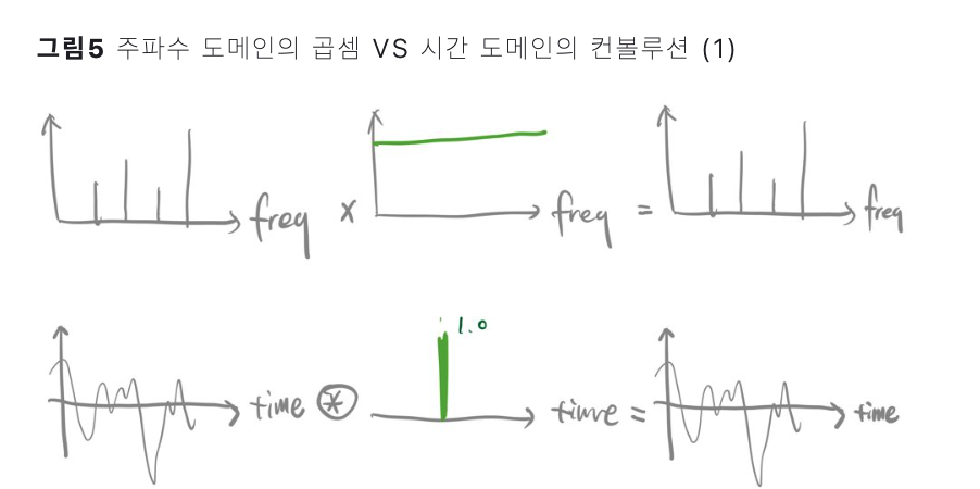
Convolution in TIME & FREQUENCY domain
(1) Standard CNN ( TIME domain )
convolutions between
- (1) the input waveform
- (2) some Finite Impulse Response (FIR) filters
\(y[n]=x[n] * h[n]=\sum_{l=0}^{L-1} x[l] \cdot h[n-l]\).
- \(x[n]\) : a chunk of the speech signal
- \(h[n]\) : the filter of length \(L\)
- \(y[n]\) : the filtered output
\(\rightarrow\) all the \(L\) elements (taps) of each filter are learned from data.
(2) CNN in SincNet
convolution with a predefined function \(g\) that depends on few learnable parameters \(\theta\) only
\(y[n]=x[n] * g[n, \theta]\).
What to use for \(g\)?
- a filter-bank composed of rectangular bandpass filters
In the frequency domain …. the magnitude of a generic bandpass filter
= difference between two low-pass filters:
- \(G\left[f, f_1, f_2\right]=\operatorname{rect}\left(\frac{f}{2 f_2}\right)-\operatorname{rect}\left(\frac{f}{2 f_1}\right)\).
- where \(f_1\) and \(f_2\) are the learned low and high cutoff frequencies
- \(\operatorname{rect}(\cdot)\) is the rectangular function in the magnitude frequency domain
Returning to the TIME domain (using the inverse Fourier transform)
\(\rightarrow\) \(g\left[n, f_1, f_2\right]=2 f_2 \sin c\left(2 \pi f_2 n\right)-2 f_1 \operatorname{sinc}\left(2 \pi f_1 n\right)\)
- where the sinc function is defined as \(\operatorname{sinc}(x)=\sin (x) / x\).
The cut-off frequencies can be initialized randomly in the range \(\left[0, f_s / 2\right]\),
- \(f_s\) : sampling frequency of the input signal
- alternative ) filters can be initialized with the cutoff frequencies of the mel-scale filter-bank
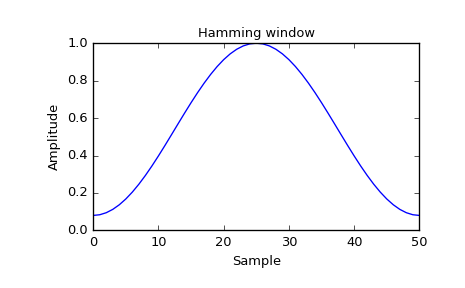
(3) Hamming window
To smooth out the abrupt discontinuities at the ends of \(g\) :
\(g_w\left[n, f_1, f_2\right]=g\left[n, f_1, f_2\right] \cdot w[n] .\).
\(\rightarrow\) use the popular Hamming window
- \(w[n]=0.54-0.46 \cdot \cos \left(\frac{2 \pi n}{L}\right)\).
3. Experiments
Datasets: Different corpora and compared to numerous speaker recognition baselines
(1) Corpora
Datasets
- TIMIT (462 spks, train chunk)
- Librispeech (2484 spks)
( Non-speech intervals at the beginning and end of each sentence were removed )
(2) Setup
[Data] Waveform of each sentence
- split into chunks of 200 ms (with 10 ms overlap)
[Architecture]
1st layer of SincNet (proposed)
- using 80 filters of length \(L = 251\) samples
2nd & 3rd layer of SincNet
- two standard CNN using 60 filters of length 5
Details
- Layer normalization
- 3 FC layers composed of 2048 neurons & BN
- leaky-ReLU
- parameters of the sinc-layer were initialized using mel-scale cutoff frequencies
(3) Baseline Setup
- standard CNN fed by raw waveform
- hand-crafted features (39 MFCCs … static + \(\Delta\) + \(\Delta \Delta\) )
4. Result
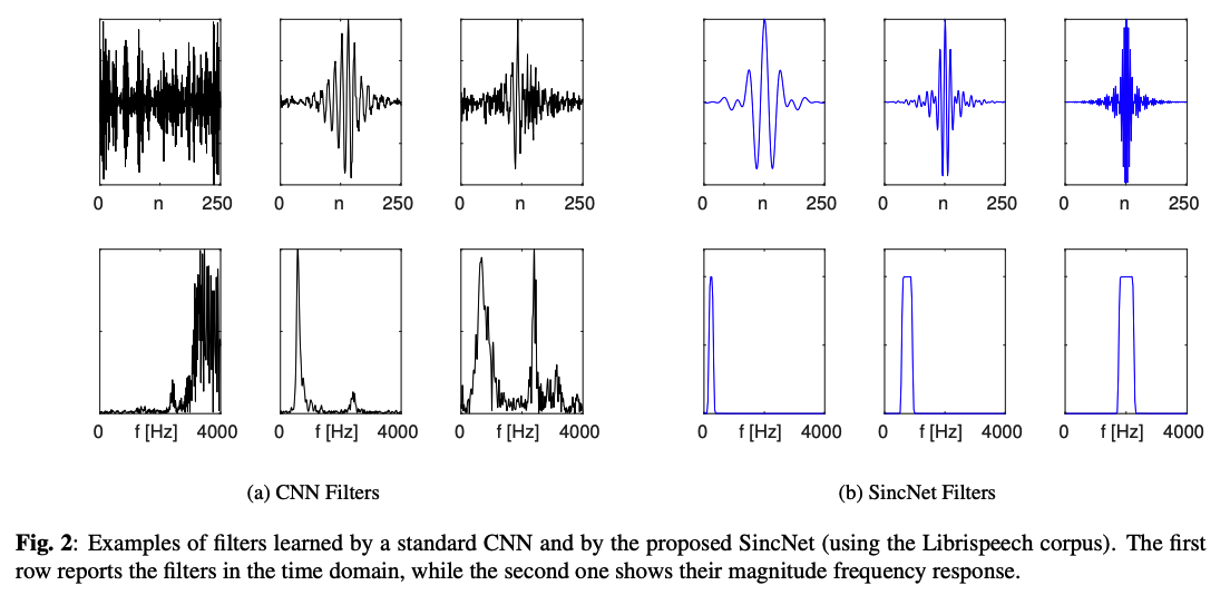
(1) Filter Analysis
(2) Speaker Identification
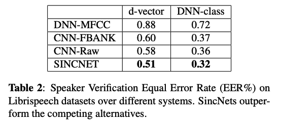
(3) Speaker Verification