Masked Spectrogram Prediction For Self-Supervised Audio Pre-Training

Masked Spectrogram Prediction For Self-Supervised Audio Pre-Training (arxiv 2022)

https://arxiv.org/pdf/2204.12768.pdf

Contents

1. Abstract
2. Masked Spectogram Prediction (MaskSepc)
   1. Masking Strategy
   2. Encoder
   3. Decoder
   4. Implementation of framework

Abstract

Limitations of previous methods

• (1) pretrain using other domaines
  • notable gap with the audio domain.
• (2) pretrain using audio domain
  • currently do not perform well in the downstream tasks.

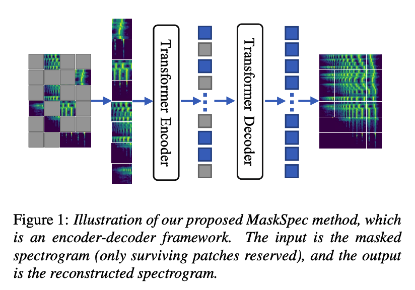
MaskSpec (masked spectrogram prediction)

• transformer-based audio models

• SSL method uusing unlabeled audio data (AudioSet)

• procedure
  • step 1) masks random patches of the input spectrogram
  • step 2) reconstructs the masked regions

1. Masked Spectogram Prediction

Why input as spectogram ( why not raw waveform [20] or others ) ?

• (1) spectrogram is sparse and contains abundant low-level acoustic information, and it has similar characteristics as the image, which has been proven to successfully adapt the transformer-based models

• (2) spectrogram input provides the SOTA for many audio tasks [16, 24]

• (3) spectrogram can be directly used as the input

  ( \(\leftrightarrow\) raw waveform often needs extra convolutional layers )

(1) Masking Strategy

Simple random mask strategy is effective and easy to implement.

Notation

• spectrogram \(\boldsymbol{T} \in \mathcal{R}^{N_t \times N_f}\)
  • where \(N_t\) and \(N_f\) denote the number of frames and the frequency bin within one frame
• training sample of dataset \(\mathcal{D}\)
• a size of \(p \times p\) sliding window with the same hop size is first applied to get the patches \(\boldsymbol{E}=\left\{e_1, \ldots, e_n\right\}\)
  • \(n\) : number of patches …. \(n=\left\lfloor\frac{N_t}{p}\right\rfloor \times\left\lfloor\frac{N_f}{p}\right\rfloor\).
• \(N=\lfloor n \times \alpha\rfloor\) : number of the masked patches,
  • \(\alpha\) : masking ratio, where \(\alpha \in[0.05,0.95]\)

Different from the previous methods such as the masked patch sampling [22] …

\(\rightarrow\) directly remove the masked patches to make the pre-training efficient & keeps the position index of all the patches for the decoder to do the reconstruction.

(2) Encoder

same encoder architecture as PaSST (i.e. PaSST-Small and PaSST-Tiny)

\(\rightarrow\) called MaskSpec, MaskSpec-Small and MaskSpec-Tiny

Encoder is composed of …

• learnable linear projection
• stack of \(N_d=12\) transformer blocks.
  • each block : \(N_h\) attention heads, \(N_{e m b}\) dimension of embedding and positionwise feed-forward network (FFN) with a hidden size of \(N_{f f n}\).

Settings

• MaskSpec : \(N_h=12, N_{e m b}=768\) and \(D_{f f n}=2048\).
• MaskSpec-Small : \(N_h=6, N_{e m b}=384\) and \(D_{f f n}=1536\).
• MaskSpec-Tiny : \(N_h=3, N_{e m b}=192\) and \(D_{f f n}=768\).

(3) Decoder

only used during pre-training ( for spectrogram reconstruction )

\(\therefore\) use a relatively lightweight decoder

( same decoder is used for MaskSpec, MaskSpec-Small and MaskSpec-Tiny )

Before feeding to decoder…

• step 1) Add masked vectors
  • ( According to the position index ) insert shared and learnable vectors into masking regions of the output of the encoder & reassemble them
• step 2) Add position info
  • inject information about the absolute position of the tokens in the sequence

Decoder is composed of …

• 8 layers of transformer blocks
  • each block : 16 attention heads with the embedding size of 512 , and the feed-forward layers have a dimensionality of 2048.
  • function of the last layer is to convert the output of the final FFN to the masked patches, in which each patch has a dimensionality of \(p \times p\).
• linear projection layer.

(4) Implementation of framework

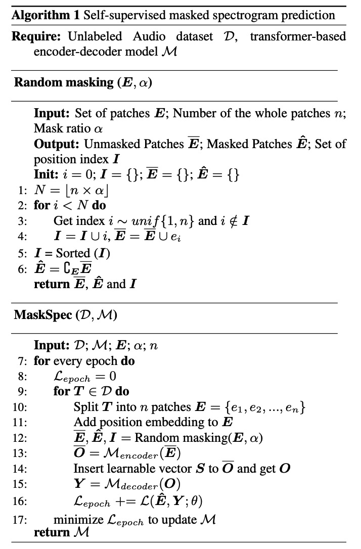
[ Encoder ]

• step 1) input spectrogram \(\boldsymbol{T}\) is split into \(n\) spectrogram patches
• step 2) add position information to patches
  • via sinusoidal position encoding
• step 3) randomly mask \(\alpha\) spectrogram patches
  • masked index = \(\boldsymbol{I}=\left\{I_1, \ldots, I_N\right\}\).
  • unmasked patches = \(\overline{\boldsymbol{E}}=\left\{e_i\right\}_{i \notin I_i}^{n-N}\)
• step 4) feed \(\overline{\boldsymbol{E}}\) into encoder
  • output of the final hidden layers : \(\overline{\boldsymbol{O}}=\left\{o_i\right\}_{i \notin I_i}^{n-N}\)

[ Decoder ]

• step 5) fill each masked patch with a learnable vector \(\boldsymbol{S} \in \mathcal{R}^{N_{e m b}}\)
  • result = input of the decoder \(\boldsymbol{O}=\left\{o_1, \ldots, o_n\right\}\).
• step 6) decoder & final linear projection layer map \(\boldsymbol{O}\) to the same dimension as the original masked patches \(\boldsymbol{E}\).

[ Loss function : MSE ]

\(\mathcal{L}(\hat{\boldsymbol{E}}, \boldsymbol{Y} ; \theta)=\sum_{i=I_1}^{I_N} \mid \mid \hat{E}_i-Y_i \mid \mid ^2\).

• masked patches \(\boldsymbol{Y}=\left\{y_{I_1}, \ldots, y_{I_N}\right\}\)
• reconstructed patches \(\hat{\boldsymbol{E}}=\left\{e_{I_1}, \ldots, e_{I_N}\right\}\)