BEATs; Audio Pre-Training with Acoustic Tokenizers

BEATs: Audio Pre-Training with Acoustic Tokenizers ( ICML 2023 )

https://arxiv.org/pdf/2212.09058.pdf

Contents

1. Abstract
2. Introduction
3. Related Work
   1. Supervised audio pre-training
   2. Self-supervised audio pre-training
   3. Audio and Speech Tokenizer
4. BEATs
   1. Iterative Audio Pre-training
   2. Acoustic Tokenizers
   3. Audio SSL Model
5. Experiments
   1. Datasets
   2. Implementation Details
   3. Comparing with SOTA single models
   4. Comparing Different BEATs Tokenizers
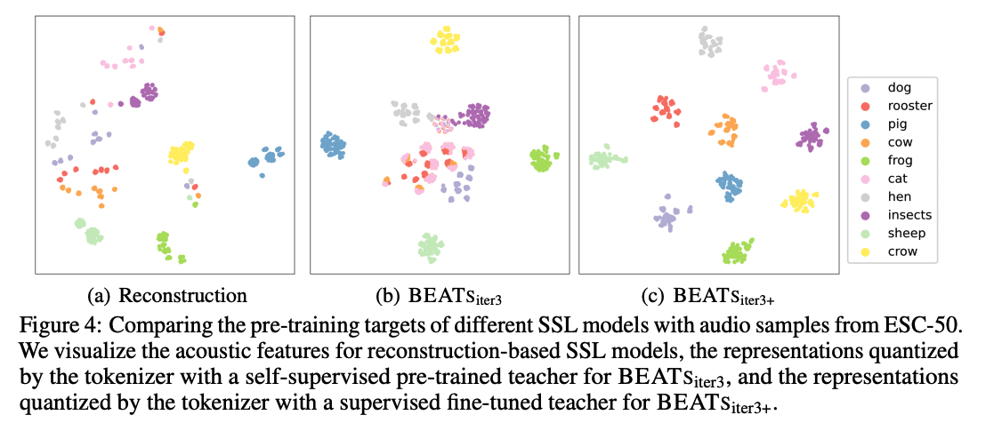
   5. Comparing Different Pre-training Targets via Visualization
   6. Comparing with SOTA Ensemble Models

Abstract

SOTA audio SSL models still employ reconstruction loss for pre-training

\(\leftrightarrow\) semantic-rich discrete label prediction encourages the SSL model to abstract the high-level audio semantics and discard the redundant details as in human perception.

Problem: semantic-rich acoustic tokenizer for general audio pre-training is usually not straightforward to obtain… because

• (1) due to the continuous property of audio
• (2) unavailable phoneme sequences like speech.

Solution: BEATs

• an iterative audio pre-training framework

  • to learn Bidirectional Encoder representation from Audio Transformers
  • (1) acoustic tokenizer and an (2) audio SSL model are optimized by iterations.

• Iteration

  • step 1) random projection as the acoustic tokenizer to train an audio SSL model in a mask and label prediction manner.
  • step 2) train an acoustic tokenizer for the next iteration by distilling the semantic knowledge from the pre-trained or fine-tuned audio SSL model.

  \(\rightarrow\) repeated with the hope of mutual promotion of the acoustic tokenizer and audio SSL model.

Experiments

• acoustic tokenizers can generate discrete labels with rich audio semantics
• BEATs acheives SOTA results across various audio classification benchmarks
  • even outperforming previous models that use more training data and model parameters significantly.
• code & pre-trained models : https://aka.ms/beats.

1. Introduction

a) Speech SSL models

• ex) Wav2vec 2.0 [Baevski et al., 2020], HuBERT [Hsu et al., 2021], BigSSL [Zhang et al., 2022], WavLM [Chen et al., 2022b], and data2vec [Baevski et al., 2022]
• show prominent performance across various speech processing tasks, especially in low-resource scenarios.

b) Speech vs Audio

• (unlike speech) audio typically contains wide variations of environmental events

  • ex) human voices, nature sounds, musical beats

  \(\rightarrow\) brings great challenges to general audio modeling.

c) Audio SSL models

• ex) SS-AST [Gong et al., 2022a], AudioMAE [Xu et al., 2022]
• proposed for general audio classification applications
• demonstrating that SSL learns robust auditory representations not only for speech but also for non-speech signals.

d) SOTA Audio SSL models [Xu et al., 2022, Chong et al., 2022]

• employ an acoustic feature reconstruction loss as the pre-training objective

  ( instead of the discrete label prediction )

• However, it was generally believed that the reconstruction loss …

  • only accounts for the correctness of low-level time-frequency features
  • but neglects high-level audio semantic abstraction

  \(\rightarrow\) Discrete label prediction would be a potentially better audio pre-training objective, for below reasons.

e) Why “Discrete Label Prediction”?

• Reason 1) From the bionics aspect, humans understand audio by extracting and clustering the high-level semantics instead of focusing on the low-level time-frequency details

• Reason 2) From the aspect of modeling efficiency,

  • [1] Reconstruction loss : waste the audio model parameter capacity and pre-training resources on predicting the semantic irrelevant information

    \(\rightarrow\) little benefit to the general audio understanding tasks.

  • [2] Discrete label prediction : provide semantic-rich tokens as the pre-training targets

    \(\rightarrow\) encourage the model to discard the redundant details

• Reason 3) Advances the unification of language, vision, speech, and audio pre-training.

  • Instead of designing the pre-training task for each modality, this unification enables the possibility of building a foundation model across modalities with a single pre-training task, i.e. discrete label prediction.

f) Challenges of of discrete label prediction in Audio

• Reason 1) Audio signal is continuous and the same acoustic event might have various durations in different occasions

  \(\rightarrow\) not straightforward to directly split the audio into semantically meaningful tokens as in language processing [Devlin et al., 2019].

• Reason 2) (Different from speech,) general audio signals contain excessively larger data variations, including various non-speech acoustic events and environmental sounds

  \(\rightarrow\) commonly used speech tokenizer for phoneme information extraction can not be directly applied

g) Solution: BEATs

BEATs = Bidirectional Encoder representation from Audio Transformers

• (1) acoustic tokenizer and an (2) audio SSL model are optimized through an iterative audio pre-training framework

  • step 1) use the acoustic tokenizer to generate the discrete labels of the unlabeled audio
    • use them to optimize the audio SSL model with a mask and discrete label prediction loss.
  • step 2) audio SSL model acts as a teacher
    • to guide the acoustic tokenizer to learn audio semantics with knowledge distillation

  \(\rightarrow\) acoustic tokenizer and the audio SSL model can benefit from each other.

h) Details

• first iteration) random-projection acoustic tokenizer

  • to generate discrete labels as a cold start.

• can fine-tune the audio SSL model with a little supervised data

  \(\rightarrow\) use the fine-tuned model as the teacher for acoustic tokenizer training.

  ( can further improve the tokenizer quality )

• compatible with any masked audio prediction model, regardless of backbone

• backbone of our audio SSL model = vanilla ViT model

  • apply the speed-up technique proposed in He et al. [2022].

• mask 75% of the input sequence

  & let the model predict the corresponding discrete labels on mask regions.

i) Experimental results

• Task: Six audio and speech classification tasks

• Result: SOTA audio understanding performance on AudioSet-2M
  • outperform the previous SOTA results by a large margin with much fewer model parameters and training data
• Demonstrate the effectiveness of our proposed acoustic tokenizers
  • generated discrete labels are robust to random disturbances and well aligned with audio semantics.

j) Contribution

• (1) Iterative audio pre-training framework
  • opens the door to audio pre-training with a discrete label prediction loss
    • better than with reconstruction loss.
  • unifies the pre-training for speech and audio
    • sheds light on the foundation model building for both speech and audio.
• (2) Effective acoustic tokenizers
  • to quantize continuous audio features into semantic-rich discrete labels
  • facilitating future work of audio pre-training and multi-modality pre-training.
• (3) SOTA results
  • on several audio and speech understanding benchmarks.

2. Related Work

(1) Supervised audio pre-training.

Either leverage (a) or (b) for pre-training

• (a) out-of-domain supervised data (e.g. ImageNet)
• (b) in-domain supervised audio data (e.g. AudioSet)

(a) Out-of-domain supervised data

• PSLA [Gong et al., 2021b]
  • use an ImageNet supervised pre-trained EfficientNet

• AST [Gong et al., 2021a], PaSST [Koutini et al., 2021], MBT [Nagrani et al., 2021] and HTS-AT [Chen et al., 2022a]

  • employ Transformer-based architectures as the backbone

  • ex) ViT [Dosovitskiy et al., 2021] and Swin Transformer [Liu et al., 2021]

(b) In-domain supervised audio data

• CLAP [Elizalde et al., 2022]
  • inspired by the vision pre-training method CLIP [Radford et al., 2021]
  • proposes a contrastive language-audio pretraining task to learn the text-enhanced audio representations with supervised audio and text pairs.
• Wav2clip [Wu et al., 2022] and Audioclip [Guzhov et al., 2022]
  • Instead of pre-training from scratch, leverage the CLIP pre-trained model and learn an additional audio encoder with the supervised pairs of audio and class labels from AudioSet.
• Some previous works: previous works [Kong et al., 2020, Verbitskiy et al., 2022, Gong et al., 2021a, Chen et al., 2022a, Koutini et al., 2021, Xu et al., 2022]
  • report the results on ESC-50 (1.6K training samples) with an additional round of supervised pre-training on the AudioSet dataset (2M training samples)
  • to push the performance for audio classification tasks with scarce data,

\(\rightarrow\) (Common) strongly rely on a great amount of supervised data,

(2) Self-supervised audio pre-training.

Only require large-scale unlabeled data

Ex) contrastive learning or reconstruction objective.

a) Contrastive Learning

• LIM [Ravanelli and Bengio, 2018], COLA [Saeed et al., 2021], Fonseca et al. [2021]
  • (pos) augmented clips from the same audio
  • (neg) ones sampled from the different audios
• CLAR [Al-Tahan and Mohsenzadeh, 2021]
  • Instead of taking only the raw waveform or the acoustic feature as the input, proposes several data augmentation methods on both of them
• Wang and Oord [2021]
  • maximize the agreement between the raw waveform and its acoustic feature

b) Reconstruction Task

Audio2Vec [Tagliasacchi et al., 2020]

• (1) CBoW task
  • reconstruct the acoustic feature of an audio clip of pre-determined duration ( based on past and future clips )
• (2) Skip-gram task
  • to predict the past and future clips ( based on the middle audio clip )

BYOL-A [Niizumi et al., 2021]

• adopts the siamese architecture as BYOL [Grill et al., 2020]
• learns to encode the robust audio representations that are invariant to different audio augmentation methods

SSAST [Gong et al., 2022a]

• proposes a patch-based SSL method to pre-train AST [Gong et al., 2021a]
• use both the (1) reconstruction and (2) contrastive loss

MSM-MAE [Niizumi et al., 2022], MaskSpec [Chong et al., 2022], MAE-AST [Baade et al., 2022] and Audio-MAE [Xu et al., 2022]

• learn the audio representations following the Transformer-based encoder-decoder design
• reconstruction pre-training task in MAE

Until now, the MAE-style reconstruction pre-training methods show SOTA

Others

Audio2Vec [Tagliasacchi et al., 2020]

• proposes the Temporal Gap pre-training task
  • estimate the absolute time distance between two audio clips
  • but inferior to the reconstruction tasks

Carr et al. [2021]

• permutation-based SSL method
  • trained to reorder the shuffled patches of an input acoustic feature,
• leverage differentiable ranking to enable end-to-end model pre-training.

(3) Audio and Speech Tokenizer

Dieleman et al. [2018]

• hierarchical VQ-VAE based model to learn audio discrete representations for music generation tasks.

HuBERT [Hsu et al., 2021]

• generates discrete labels with the iterative hidden state clustering method for speech SSL task

  ( = hidden state is extracted from the last round speech SSL model )

Chiu et al. [2022]

• claim a random-projection tokenizer is adequate for a large speech SSL model pre-training.

Proposed BEATs:

• first to train an acoustic tokenizer with the supervision of the last round SSL model

  ( different from the previous auto-encoding and ad-hoc clustering methods )

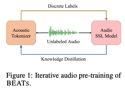
3. BEATs

(1) Iterative Audio Pre-training

( Until convergence … )

Given the unlabeled audio, use the acoustic tokenizer to generate the discrete labels, and use them to train the audio SSL model with a mask and discrete label prediction loss.

( After convergence … )

use the audio SSL model as the teacher to train a new acoustic tokenizer with knowledge distillation for the next iteration of audio SSL model training.

Settings

Input: Audio clip \(\rightarrow\) extract Acoustic Features

• split them into regular grid patches

  & flatten them to the patch sequence \(\mathbf{X}=\left\{\mathbf{x}_t\right\}_{t=1}^T\).

Acoustic tokenizer

• quantize the patch sequence \(\mathbf{X}\) to the patch-level discrete labels \(\hat{Z}=\left\{\hat{z}_t\right\}_{t=1}^T\) as the masked prediction targets.

Audio SSL model

• encode the patch sequence \(\mathbf{X}\) and extract the output sequence \(\hat{\mathbf{O}}=\left\{\hat{\mathbf{o}}_t\right\}_{t=1}^T\) as the knowledge distillation targets.

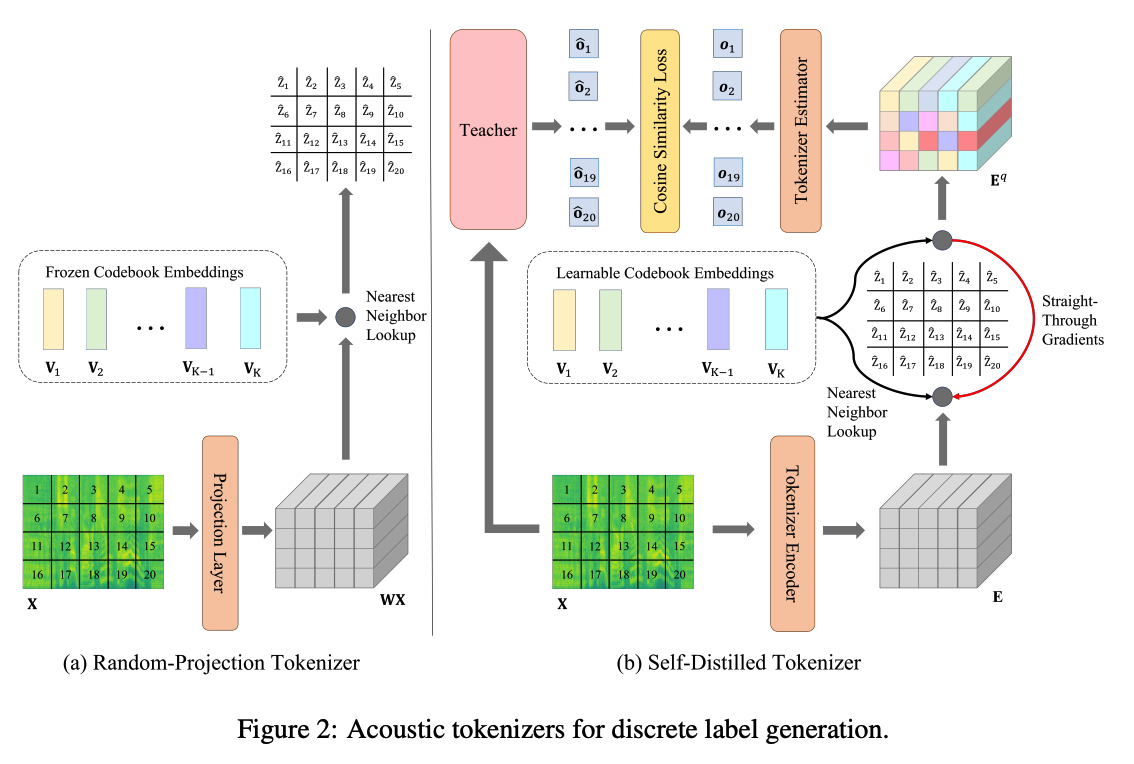
(2) Acoustic Tokenizers

First iteration )

• teacher model is unavailable
• employ a Random-Projection Tokenizer (Section 3.2.1) to cluster the continuous acoustic features into discrete labels as a cold start

Second iteration ~ )

• train a Self-Distilled Tokenizer (Section 3.2.2) to generate the refined discrete labels with the semantic-aware knowledge distilled from the pre-trained/fine-tuned audio SSL model obtained in the last iteration

a) Cold Start: Random-Projection Tokenizer

Apply the random-projection tokenizer to generate the patch-level discrete labels for each input audio.

Random-projection tokenizer

• linear projection layer & a set of codebook embeddings
  • kept frozen after random initialization.

Procedure

• input: patch sequence extracted from the input audio \(\mathbf{X}=\left\{\mathbf{x}_t\right\}_{t=1}^T\),
• step 1) Project \(\mathbf{x}_t\) to the vector \(\mathbf{W} \mathbf{x}_t\)
  • with a randomly initialized projection layer \(\mathbf{W}\).
• step 2) Look up the nearest neighbor vector of each projected vector \(\mathbf{W} \mathbf{x}_t\)
  • from a set of random initialized vectors \(\mathbf{V}=\left\{\mathbf{v}_i\right\}_{i=1}^K\),
    • where \(K\) is the codebook size
• step 3) Define the discrete label of \(t\)-th patch as the index of the nearest neighbor vector
  • \(\hat{z}_t=\underset{i}{\arg \min } \mid \mid \mathbf{v}_i-\mathbf{W} \mathbf{x}_t \mid \mid _2^2\).

b) Iteration: Self-Distilled Tokenizer

Self-distilled tokenizer

• Leverage the last iteration audio SSL model as the teacher ( can be either a pre-trained model or a fine-tuned model ) to teach the current iteration tokenizer learning.

Procedure

• step 1) Encode: uses a Transformer-based tokenizer encoder
  • convert the input patches to discrete labels with a set of learnable codebook embeddings
  • input: \(\mathbf{X}=\left\{\mathbf{x}_t\right\}_{t=1}^T\)
  • ouutput : \(\mathbf{E}=\left\{\mathbf{e}_t\right\}_{t=1}^T\)
• step 2) Nearest Neighbor
  • quantization by finding the nearest neighbor vector \(\mathbf{v}_{\hat{z}_t}\) from the codebook embeddings \(\mathbf{V}=\left\{\mathbf{v}_i\right\}_{i=1}^K\)
  • \(\hat{z}_t=\underset{i}{\arg \min } \mid \mid \ell_2\left(\mathbf{v}_i\right)-\ell_2\left(\mathbf{e}_t\right) \mid \mid _2^2\).
• step 3) Predict: trained to predict the output of a teacher model
  • input: discrete labels and codebook embeddings
  • use 3-layer Transformer estimator to predict the last layer output of the teacher model \(\left\{\hat{\mathbf{o}}_t\right\}_{t=1}^T\).
  • tokenized discrete labels are optimized to contain more semantic rich knowledge from the teacher and less redundant information of the input audio

c) Overall training objective

Objective of the self-distilled tokenizer

• cosine similarity between ..
  • (1) the output sequence of the tokenizer estimator \(\left\{\mathbf{o}_t\right\}_{t=1}^T\)
  • (2) the output sequence of the teacher model \(\left\{\hat{\mathbf{o}}_t\right\}_{t=1}^T\),
• the mean squared error between ..
  • (1) the encoded vector sequence \(\mathbf{E}=\left\{\mathbf{e}_t\right\}_{t=1}^T\)
  • (2) the quantized vector sequence \(\mathbf{E}^q=\left\{\mathbf{v}_{\hat{z}_t}\right\}_{t=1}^T\)

\(\max \sum_{\mathbf{X} \in \mathcal{D}} \sum_{t=1}^T \cos \left(\mathbf{o}_t, \hat{\mathbf{o}}_t\right)- \mid \mid s g\left[\ell_2\left(\mathbf{e}_t\right)\right]-\ell_2\left(\mathbf{v}_{\hat{z}_t}\right) \mid \mid _2^2- \mid \mid \ell_2\left(\mathbf{e}_t\right)-s g\left[\ell_2\left(\mathbf{v}_{\hat{z}_t}\right)\right] \mid \mid _2^2\).

Details

• employ the EMA [Van Den Oord et al., 2017] for codebook embedding optimization for more stable tokenizer training [Peng et al., 2022].

• (inference) we discard the tokenizer estimator & leverage the pre-trained tokenizer encoder and codebook embeddings to convert each input audio \(\mathbf{X}=\left\{\mathbf{x}_t\right\}_{t=1}^T\) to patch-level discrete labels \(\hat{Z}=\left\{\hat{z}_t\right\}_{t=1}^T\),

(3) Audio SSL Model

a) Backbone

ViT structure [Dosovitskiy et al., 2021]

• [Input] patch sequence extracted from the input audio \(\mathbf{X}=\left\{\mathbf{x}_t\right\}_{t=1}^T\)

• [Patch embeddings] convert them to the patch embeddings \(\mathbf{E}=\left\{\mathbf{e}_t\right\}_{t=1}^T\)

  • with a linear projection network.

• [Patch representations] feed tehm to Transformer encoder layers and obtain \(\mathbf{R}=\left\{\mathbf{r}_t\right\}_{t=1}^T\).

  Transformers are equipped with …

  • (1) a convolution-based relative position embedding layer at the bottom
  • (2) gated relative position bias [Chi et al., 2022] for better position information encoding.
  • (3) DeepNorm [Wang et al., 2022a] for more stable pre-training.

b) Pre-training

Masked Audio Modeling (MAM) task

• optimized to predict the patch-level discrete labels generated by the acoustic tokenizers with a Transformer-based label predictor

Notation

• patch sequence \(\mathbf{X}=\left\{\mathbf{x}_t\right\}_{t=1}^T\)
• corresponding target discrete acoustic labels \(\hat{Z}=\left\{\hat{z}_t\right\}_{t=1}^T\),

[Masking] randomly mask \(75 \%\) of the input patches

• positions are denoted as \(\mathcal{M}=\{1, \ldots, T\}^{0.75 T}\)

Procedure

• Step 1) masking

• Step 2) Feed the unmasked patch sequence \(\mathbf{X}^U=\left\{\mathbf{x}_t: t \notin \mathcal{M}\right\}_{t=1}^T\) to the ViT encoder
  • obtain the encoded representations \(\mathbf{R}^U=\left\{\mathbf{r}_t: t \notin \right.\) \(\mathcal{M}\}_{t=1}^T\).
• Step 3) Feed the combination of the non-masked patch representations and the masked patch features \(\left\{\mathbf{r}_t: t \notin \mathcal{M}\right\}_{t=1}^T \cup\{\mathbf{0}: t \in \mathcal{M}\}_{t=1}^T\) to the label predictor
  • predict the discrete acoustic labels \(Z=\left\{z_t\right\}_{t=1}^T\).
  • Only feed the non-masked patches into the encoder \(\rightarrow\) significantly speed up

Pretraining objective : CE loss

• \(\mathcal{L}_{\mathrm{MAM}}=-\sum_{t \in \mathcal{M}} \log p\left(\hat{z}_t \mid \mathbf{X}^U\right)\).

c) Fine-Tuning

• discard the label predictor,

• append a task-specific linear classifier

  • to generate the labels for the downstream classification tasks,

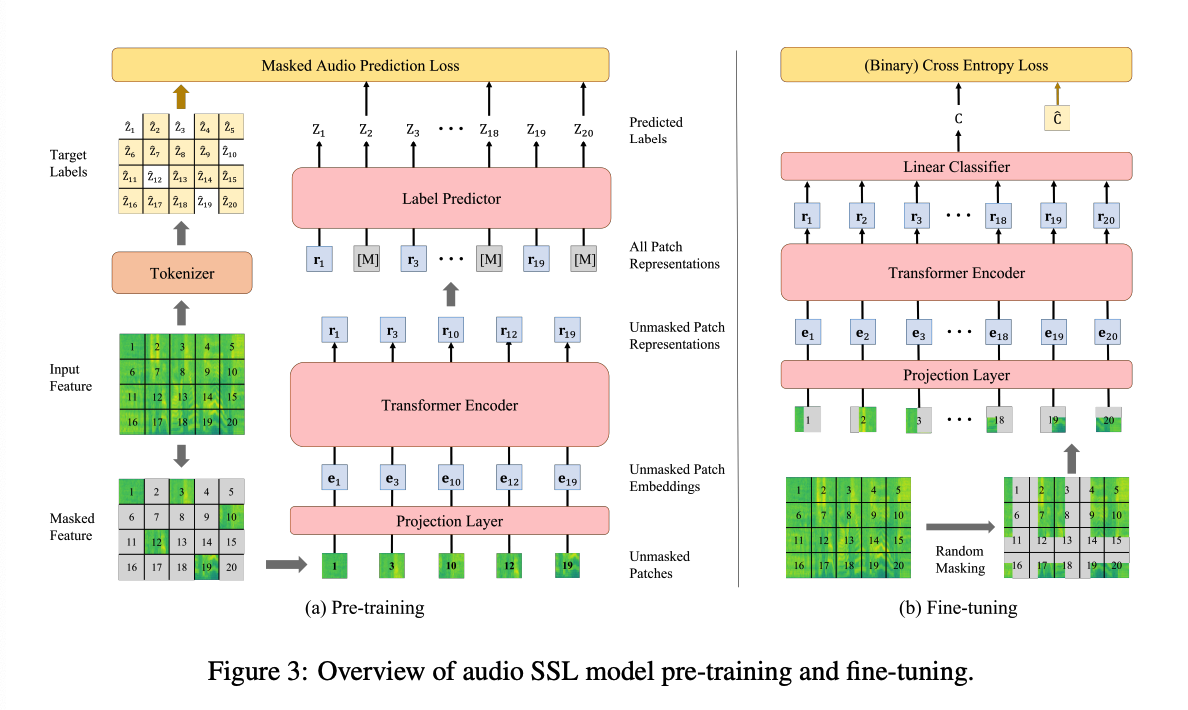
Procedure

• Step 1) Randomly mask the input acoustic feature
  • in the time and frequency dimension as spec-augmentation [Park et al., 2019]
• Step 2) Split and flat it to the patch sequence \(\mathbf{X}=\left\{\mathbf{x}_t\right\}_{t=1}^T\).
• Step 3) Feed the whole patch sequence \(\mathbf{X}\) to the ViT encoder & obtain \(\mathbf{R}=\left\{\mathbf{r}_t\right\}_{t=1}^T\).
• Step 4) \(p(C)=\operatorname{Softmax}\left(\operatorname{MeanPool}\left(\mathbf{W}_c \mathbf{R}\right)\right)\).

Loss function

• CE loss : for the single label classification tasks
• BCE loss : for the multi-label classification tasks or the mixup augmentation is employed.

4. Experiments

(1) Datasets

pass

(2) Implementation Details

a) Backbone

• 12 Transformer encoder layers

• 768-dimensional hidden states

• 8 attention heads

\(\rightarrow\) 90M parameters

( keep the model size similar to the previous SOTA audio pre-trained models )

b) Acoustic Feature

step 1) Convert the sample rate of each raw waveform to 16,000

step 2) Extract the 128-dimensional Mel-filter bank features

• with a 25ms Povey window that shifts every 10 ms as the acoustic feature.

step 3) Normalize the acoustic feature \(N(0,0.5^2)\)

step 4) Split each acoustic feature into the 16 × 16 patches & flatten

c) Model & Tokenizer Training

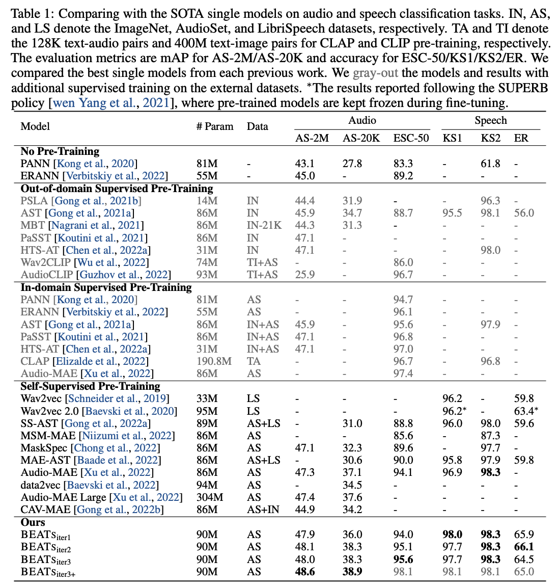
Pretrain on AS-2M dataset for 3 iterations

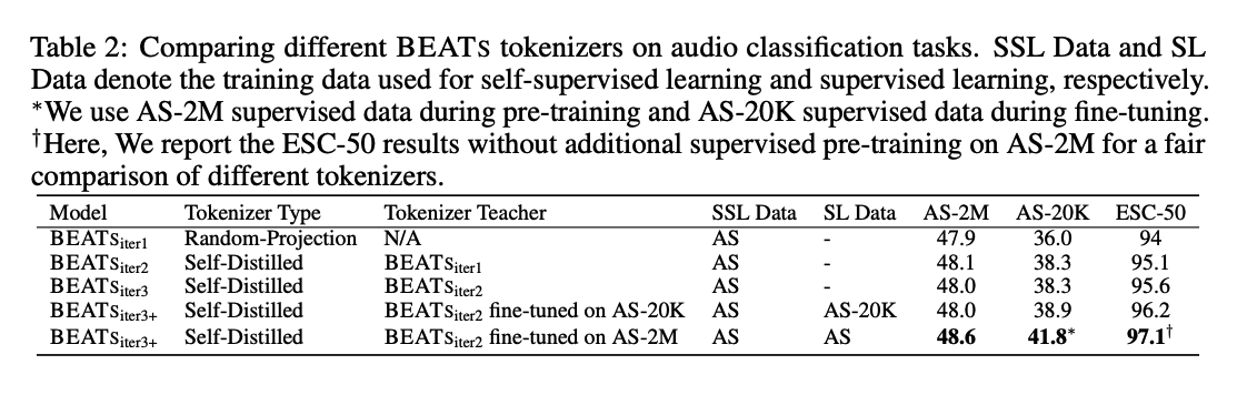
BEATs \(_{\text {iter1}}\), BEATs \(_{\text {iter2 }}\), BEATs \(_{\text {iter3 }}\), BEATs \(_{\text {iter3+ }}\).

• BEATs \(_{\text {iter1}}\) : pre-trained with the discrete labels generated by a random-projection tokenizer
• BEATs \(_{\text {iter3+ }}\) : self-distilled tokenizer for pre-training takes the supervised fine-tuned BEATs \(_{\text {iter2}}\) as the teacher model &* learns to estimate the classification logits of the input audios.

BEATs \(_{\text {iter3+ }}\) : not only make use of the downstream supervised data during fine-tuning but also in pre-training.

Other details:

• BEATS models
  • train for 400k steps with a batch size of 5.6K seconds and a 5e-4 peak learning rate.
• Codebook of all the tokenizers
  • contains 1024 embeddings with 256 dimensions
• Self-distilled tokenizer with a SSL model as the teacher
  • train for 400k steps with a batch size of 1.4K seconds and a 5e-5 peak learning rate.
• Self-distilled tokenizer with a SL model as the teacher
  • train for 400k steps with a batch size of 1.4K seconds and a 5e-4 peak learning rate.

(3) Comparing with SOTA single models

(4) Comparing Different BEATs Tokenizers

(5) Comparing Different Pre-training Targets via Visualization

(6) Comparing with the SOTA Ensemble Models