73.SLANG, Fast Structured Covariance Approximations for Bayesian Deep Learning with Natural Gradient

SLANG, Fast Structured Covariance Approximations for Bayesian Deep Learning with Natural Gradient (NeurIPS 2018)

Abstract

Uncertainty estimation : computationally challenging task!

• usually resort to a diagonal approximation of the covariance matrix

• propose SLANG!

SLANG

• **new stochastic, low-rank, approximate natural-gradient **for VI in large, deep models

1. Introduction

goal of Bayesian DL

• provide uncertainty estimates, by integrating over the posterior distn of the parameter
• but complexity of DL makes it hard…

MCMC & VI … each has its own pros and cons

\(\rightarrow\) fast and accurate estimation of uncertainty is essential!

Propose a new VI method, called “SLANG”

• SLANG = Stochastic Low-rank Approximate Natural Gradient

• to estimate Gaussian approximations with a diagonal plus low-rank covariance structure!

2. Gaussian Approximation with Natural-Gradient Variational Inference

goal : estimate uncertainties in DL using Bayesian INference

Structure

• likelihood : \(p\left(\mathcal{D}_{i} \mid \theta\right)\)
• prior distribution :
  • Gaussian \(p(\theta)\) ( ex. isotropic Gaussian, \(p(\theta) \sim \mathcal{N}(0,(1 / \lambda) \mathbf{I})\) )
• posterior :
  • requires computation of “marginal likelihood”

VI simplifies this problem! maximize ELBO

• ELBO : \(\quad \mathcal{L}(\mu, \Sigma):=\mathbb{E}_{q}[\log p(\mathcal{D} \mid \theta)]-\mathbb{D}_{K L}[q(\theta) \mid \mid p(\theta)]\)

optimize \(L\) : using stochastic gradient methods

• natural-gradients are preferable ( faster convergence )

Extend VOGN (Variaitonal Online Gauss-Newton)

Updating Equation :

• \(\boldsymbol{\mu}_{t+1}=\boldsymbol{\mu}_{t}-\alpha_{t} \boldsymbol{\Sigma}_{t+1}\left[\hat{\mathrm{g}}\left(\boldsymbol{\theta}_{t}\right)+\lambda \boldsymbol{\mu}_{t}\right]\).
• \(\boldsymbol{\Sigma}_{t+1}^{-1}=\left(1-\beta_{t}\right) \boldsymbol{\Sigma}_{t}^{-1}+\beta_{t}\left[\hat{\mathbf{G}}\left(\boldsymbol{\theta}_{t}\right)+\lambda \mathbf{I}\right]\).

where

• \(\hat{\mathrm{g}}\left(\boldsymbol{\theta}_{t}\right):=-\frac{N}{M} \sum_{i \in \mathcal{M}} \mathrm{g}_{i}\left(\boldsymbol{\theta}_{t}\right)\).
• \(\hat{\mathbf{G}}\left(\boldsymbol{\theta}_{t}\right):=-\frac{N}{M} \sum_{i \in \mathcal{M}} \mathbf{g}_{i}\left(\boldsymbol{\theta}_{t}\right) \mathbf{g}_{i}\left(\boldsymbol{\theta}_{t}\right)^{\top}\).
• \(t\) : iteration number
• \(\alpha_t, \beta_t\) : learning rates
• \[\boldsymbol{\theta}_{t} \sim \mathcal{N}\left(\boldsymbol{\theta} \mid \boldsymbol{\mu}_{t}, \boldsymbol{\Sigma}_{t}\right)\]
• \[\mathbf{g}_{i}\left(\boldsymbol{\theta}_{t}\right):=\nabla_{\theta} \log p\left(\mathcal{D}_{i} \mid \boldsymbol{\theta}_{t}\right)\]
• \(\hat{\mathbf{G}}\left(\boldsymbol{\theta}_{t}\right)\) : Empirical Fisher (EF) matrix
• \(M\) : minibatch of M data examples

Pros and Cons of VOGN

• pros) advantage of \(\boldsymbol{\Sigma}_{t+1}^{-1}=\left(1-\beta_{t}\right) \boldsymbol{\Sigma}_{t}^{-1}+\beta_{t}\left[\hat{\mathbf{G}}\left(\boldsymbol{\theta}_{t}\right)+\lambda \mathbf{I}\right]\) :
  • only requires back-propagated gradients
• cons) “approximate” ( not exact ) natural gradient

\[\boldsymbol{\Sigma}_{t+1}^{-1}=\left(1-\beta_{t}\right) \boldsymbol{\Sigma}_{t}^{-1}+\beta_{t}\left[\hat{\mathbf{G}}\left(\boldsymbol{\theta}_{t}\right)+\lambda \mathbf{I}\right]\]

• requires the storage & inversion of \(D \times D\) cov matrix

• Mean Field assumption : restrict \(\Sigma\) to be diagonal

  ( but poor approximation )

• SLANG :

  Estimate a low-rank plus diagonal approximation of $$\Sigma that reduces the computational cost,

  while still preserving some off-diagonal covariance structure

3. Stochastic, Low-rank, Approximate Natural-Gradient (SLANG) Method

Goal : modify \(\boldsymbol{\Sigma}_{t+1}^{-1}=\left(1-\beta_{t}\right) \boldsymbol{\Sigma}_{t}^{-1}+\beta_{t}\left[\hat{\mathbf{G}}\left(\boldsymbol{\theta}_{t}\right)+\lambda \mathbf{I}\right]\)

• make its time & space complexity LINEAR in \(D\)

• propose to “approximate the inverse of \(\Sigma_t\) by low-rank plus diagonal matrix”

  \(\boldsymbol{\Sigma}_{t}^{-1} \approx \hat{\boldsymbol{\Sigma}}_{t}^{-1}:=\mathbf{U}_{t} \mathbf{U}_{t}^{\top}+\mathbf{D}_{t}\).

  where \(\mathbf{U}_{t}\) is a \(D \times L\) matrix with \(L \ll D\) and \(\mathbf{D}_{t}\) is a \(D \times D\) diagonal matrix.

\(\boldsymbol{\Sigma}_{t}^{-1} \approx \hat{\boldsymbol{\Sigma}}_{t}^{-1}:=\mathbf{U}_{t} \mathbf{U}_{t}^{\top}+\mathbf{D}_{t}\).

• how to derive an updating equation for \(\mathbf{U}_{t}\) and \(\mathbf{D}_{t}\) ?

approximation to the update of \(\Sigma_{t+1}^{-1}\) :

• \(\hat{\Sigma}_{t+1}^{-1}:=\mathbf{U}_{t+1} \mathbf{U}_{t+1}^{\top}+\mathbf{D}_{t+1} \approx\left(1-\beta_{t}\right) \hat{\Sigma}_{t}^{-1}+\beta_{t}\left[\hat{\mathbf{G}}\left(\theta_{t}\right)+\lambda \mathbf{I}\right]\).

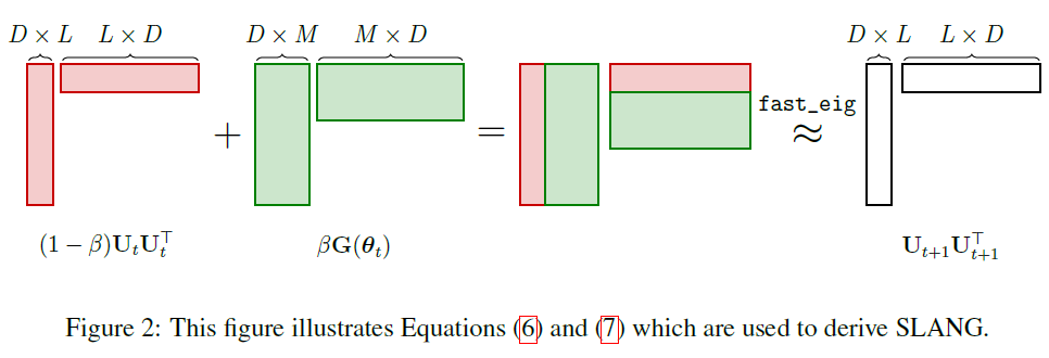
\(\begin{aligned}\left(1-\beta_{t}\right) \hat{\Sigma}_{t}^{-1}+\beta_{t}\left[\hat{\mathbf{G}}\left(\boldsymbol{\theta}_{t}\right)+\lambda \mathbf{I}\right]&=\underbrace{\left(1-\beta_{t}\right) \mathbf{U}_{t} \mathbf{U}_{t}^{\top}+\beta_{t} \hat{\mathbf{G}}\left(\boldsymbol{\theta}_{t}\right)}_{\text {Rank at most } L+M}+\underbrace{\left(1-\beta_{t}\right) \mathbf{D}_{t}+\beta_{t} \lambda \mathbf{I}}_{\text {Diagonal component }} \\ &\approx \underbrace{\mathbf{Q}_{1: L} \boldsymbol{\Lambda}_{1: L} \mathbf{Q}_{1: L}^{\top}}_{\text {Rank } L \text { approximation }}+\underbrace{\left(1-\beta_{t}\right) \mathbf{D}_{t}+\beta_{t} \lambda \mathbf{I}}_{\text {Diagonal component }}\end{aligned}\).

• 1st term = structured component
  • \(\mathbf{Q}_{1: L}\) = \(D \times L\) matrix containing first \(L\) leading eigenvectors of \(\left(1-\beta_{t}\right) \mathbf{U}_{t} \mathbf{U}_{t}^{\prime}+\beta_{t} \hat{\mathbf{G}}\left(\boldsymbol{\theta}_{t}\right)\)
  • \(\Lambda_{1: L}\) is an \(L \times L\) corresponding matrix
• 2nd term = diagonal component

\(\mathbf{U}_{t+1}=\mathbf{Q}_{1: L} \mathbf{\Lambda}_{1: L}^{1 / 2}\).

[Conclusion] update \(\mathbf{D_{t+1}}\) using diagonal correction \(\Delta_{t}\)

\(\begin{aligned} \mathrm{D}_{t+1} &=(1-\beta) \mathbf{D}_{t}+\beta_{t} \lambda \mathbf{I}+\Delta_{t} \\ \Delta_{t} &=\operatorname{diag}\left[(1-\beta) \mathbf{U}_{t} \mathbf{U}_{t}^{\top}+\beta_{t} \hat{\mathbf{G}}\left(\boldsymbol{\theta}_{t}\right)-\mathbf{U}_{t+1} \mathbf{U}_{t+1}^{\top}\right] \end{aligned}\).

New Covariance Approximation can now be used to update \(\mu_{t+1}\)

\(\text { SLANG: } \quad \mu_{t+1}=\mu_{t}-\alpha_{t}\left[\mathbf{U}_{t+1} \mathbf{U}_{t+1}^{\top}+\mathbf{D}_{t+1}\right]^{-1}\left[\hat{\mathbf{g}}\left(\theta_{t}\right)+\lambda \mu_{t}\right]\).

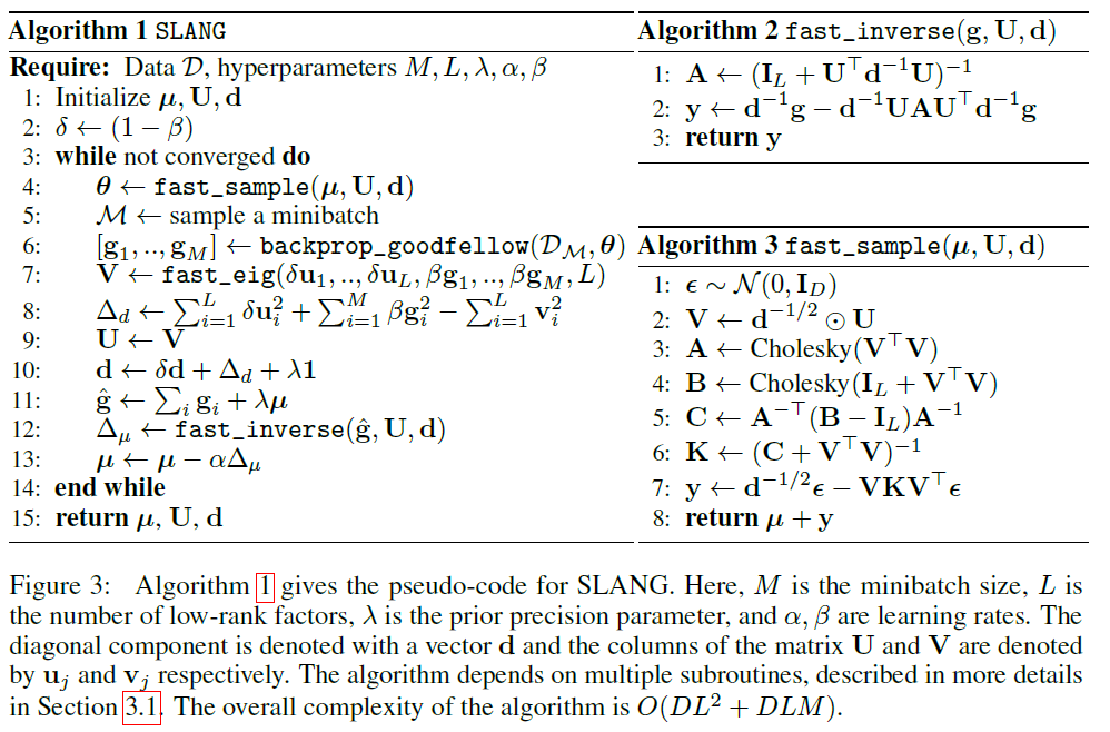
3-1. Details of SLANG

(1) every iteration, generate \(\boldsymbol{\theta}_{t} \sim \mathcal{N}\left(\boldsymbol{\theta} \mid \boldsymbol{\mu}_{t}, \mathbf{U}_{t} \mathbf{U}_{t}^{\top}+\mathbf{D}_{t}\right)\).

• reparameterization trick

• \[\boldsymbol{\theta}_{t}=\boldsymbol{\mu}_{t}+\mathbf{A}_{t} \boldsymbol{\epsilon}\]

• where \(\mathbf{A}_{t}=\left(\mathbf{U}_{t} \mathbf{U}_{t}^{\top}+\mathbf{D}_{t}\right)^{-1 / 2}\)

  and \(\boldsymbol{\epsilon} \sim \mathcal{N}(\mathbf{0}, \mathbf{I})\).

• to generate \(S\) samples, require \(O\left(D L^{2}+D L S\right)\).

(2) need to compute and store all individual stochastic gradients \(\mathrm{g}_{i}\left(\theta_{t}\right)\).

• backprop_goodfellow

(3) compute the eigenvalue decomposition of \(\left(1-\beta_{t}\right) \mathbf{U}_{t} \mathbf{U}_{t}+\beta_{t} \hat{\mathbf{G}}\left(\boldsymbol{\theta}_{t}\right)\).

• fast_eig
• computes the top- \(L\) eigendecomposition of a low-rank matrix

Overall complexity : \(O\left(D L^{2}+D L M S\right)\).

Memory cost : \(O(D L+D M S)\)