85.A Simple Baseline for Bayesian Uncertainty in Deep Learning

A Simple Baseline for Bayesian Uncertainty in Deep Learning ( NeurIPS 2019 )

Abstract

SWAG ( =SWA-Gaussian ) : simple, scalable, general purpose approach for…

• (1) uncertainty representation
• (2) calibration in deep learning

1. Introduction

Representing Uncertainty is crucial.

This paper…

• use the information contained in the SGD trajectory to efficiently approximate the posterior distn over the weights of NN
• find that “Gaussian distn” fitted to the first 2 moments of SGD captures the local geometry of posterior!

2. Related Work

2-1. Bayesian Methods

MCMC

• HMC (Hamiltonian Monte Carlo)
• SGHMC (stochastic gradient HMC)
  • allows for stochastic gradients to be used in Bayesian Inference
  • (crucial for both scalability & exploring a space of solutions to provide good generalization)
• SGLD (stochastic gradient Langevin dynamics)

Variational Inference

• Reparameterization Trick

Dropout Variational Inference

• spike and slab variational distribution
• optimize dropout probabilities as well

Laplace Approximation

• assume a Gaussian posterior, \(\mathcal{N}\left(\theta^{*}, \mathcal{I}\left(\theta^{*}\right)^{-1}\right)\).
  • \(\mathcal{I}\left(\theta^{*}\right)^{-1}\) : inverse of the Fisher information matrix

2-2. SGD based approximation

• averaged SGD as an MCMC sampler

2-3. Methods for Calibration of DNNs

(SSDE) Ensembles of several networks

3. SWA-Gaussian for Bayesian Deep Learning

propose SWAG for Bayesian model averaging & uncertainty estimation

3-1. Stochastic Gradient Descnet (SGD)

standard training of DNNs

\(\Delta \theta_{t}=-\eta_{t}\left(\frac{1}{B} \sum_{i=1}^{B} \nabla_{\theta} \log p\left(y_{i} \mid f_{\theta}\left(x_{i}\right)\right)-\frac{\nabla_{\theta} \log p(\theta)}{N}\right)\).

• loss function : NLL & regularizer
  • NLL : \(-\sum_{i} \log p\left(y_{i} \mid f_{\theta}\left(x_{i}\right)\right)\)
  • regularizer : \(\log p(\theta)\)

3-2. Stochastic Weight Averaging (SWA)

main idea of SWA

• run SGD with a constant learning rate schedule,

  starting from a pre-trained solution & average the weights

• \(\theta_{\text {SWA }}=\frac{1}{T} \sum_{i=1}^{T} \theta_{i}\).

3-3. SWAG-Diagonal

simple diagonal format for the covariance matrix.

maintain a running average of the 2nd uncentered moment for each weight,

then compute the covariance using the following standard identity at the end of training:

• \(\overline{\theta^{2}}=\frac{1}{T} \sum_{i=1}^{T} \theta_{i}^{2}\) .
• \(\Sigma_{\text {diag }}=\operatorname{diag}\left(\overline{\theta^{2}}-\theta_{\text {SWA }}^{2}\right)\).
• Approximate posterior distribution : \(\mathcal{N}\left(\theta_{\mathrm{SWA}}, \Sigma_{\text {Diag }}\right)\)

3-4. SWAG : Low Rank plus Diagonal Covariance Structure

full SWAG algorithm

• diagonal covariance approximation : TOO restrictive
• more flexible low-rank plus diagonal posterior approximation

sample covariance matrix of SGD :

• sum of outer products

• \(\Sigma=\frac{1}{T-1} \sum_{i=1}^{T}\left(\theta_{i}-\theta_{\mathrm{SWA}}\right)\left(\theta_{i}-\theta_{\mathrm{SWA}}\right)^{\top}\) ( rank = \(T\) )

  • but don’t know \(\theta_{SWA}\) during training

• \(\Sigma \approx \frac{1}{T-1} \sum_{i=1}^{T}\left(\theta_{i}-\bar{\theta}_{i}\right)\left(\theta_{i}-\right.\left.\bar{\theta}_{i}\right)^{\top}=\frac{1}{T-1} D D^{\top}\).

  • where \(D\) is the deviation matrix comprised of columns \(D_{i}=\left(\theta_{i}-\bar{\theta}_{i}\right)\)

    and \(\bar{\theta}_{i}\) is the running estimate of the parameters’ mean obtained from the first \(i\) samples

Combine (1) & (2)

• (1) low-rank approximation : \(\Sigma_{\text {low-rank }}=\frac{1}{K-1} \cdot \widehat{D} \widehat{D}^{\top}\)
• (2) diagonal approximation : \(\Sigma_{\text {diag }}=\operatorname{diag}\left(\overline{\theta^{2}}-\theta_{\text {SWA }}^{2}\right)\)

\(\rightarrow\) \(\mathcal{N}\left(\theta_{\text {SWA }}, \frac{1}{2} \cdot\left(\Sigma_{\text {diag }}+\Sigma_{\text {low-rank }}\right)\right)\).

To sample from SWAG, we use….

• \(\tilde{\theta}=\theta_{\mathrm{SWA}}+\frac{1}{\sqrt{2}} \cdot \Sigma_{\mathrm{diag}}^{\frac{1}{2}} z_{1}+\frac{1}{\sqrt{2(K-1)}} \widehat{D} z_{2}\).

  where \(z_{1} \sim \mathcal{N}\left(0, I_{d}\right), z_{2} \sim \mathcal{N}\left(0, I_{K}\right)\).

Full Algorithm

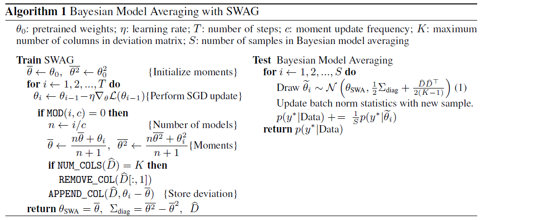
3-5. Bayesian Model Averaging with SWAG

MAP

• posterior \(\log p(\theta \mid \mathcal{D})=\log p(\mathcal{D} \mid \theta)+\log p(\theta)\).
• prior \(p(\theta)\) : regularization in optimization

Bayesian procedure “marginalizes” the posterior over \(\theta\)

• \(p\left(y_{*} \mid \mathcal{D}, x_{*}\right)=\int p\left(y_{*} \mid \theta, x_{*}\right) p(\theta \mid \mathcal{D}) d \theta\).

• using MC sampling…

  \(p\left(y_{*} \mid \mathcal{D}, x_{*}\right) \approx \frac{1}{T} \sum_{t=1}^{T} p\left(y_{*} \mid \theta_{t}, x_{*}\right), \quad \theta_{t} \sim p(\theta \mid \mathcal{D})\).

Prior Choice

• (typically) weight decay is used to regularize DNN

• when SGD is used with momentum \(\rightarrow\) implicit regularization