Variational Inference

( 이론 참고 : https://seunghan96.github.io/bnn )

( 코드 참고 : https://www.ritchievink.com/blog/2019/09/16/variational-inference-from-scratch/ )

1. Import Packages

Variational Inference 구현을 위한 주요 패키지들을 불러온다. ( Pytorch, Numpy … )

import torch
import torch.nn as nn
import torch.nn.functional as F
import torch.distributions as dist
import matplotlib.pyplot as plt
from dataclasses import dataclass
import numpy as np

GPU 사용 여부

torch.tensor( ).to(device)를 계속 사용하는 것을 피하기 위해

Tensor = torch.cuda.FloatTensor를 사용한다.

cuda = True if torch.cuda.is_available() else False
Tensor = torch.cuda.FloatTensor if cuda else torch.FloatTensor

2. 가상 데이터 생성

아래와 같은 임의의 데이터를 생성한다.

Y_real : noise가 없는 Y
Y_noise : Y_real에 \(\epsilon \sim N(0,\sigma)\)의 noise가 낀 값

def func(x):
    return 0.2*np.power(x, 3)-2*np.power(x, 2+1)+8*x

n=10000
sigma=1.5

X = np.linspace(-3, 3, n)
Y_real = func(X)
Y_noise = (Y_real+np.random.normal(0,sigma,n))

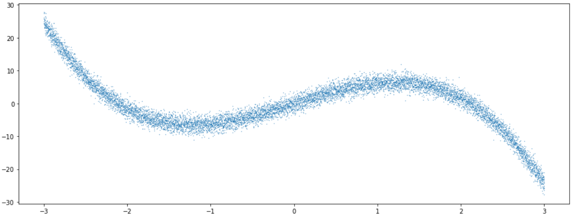
데이터의 모양을 보면 아래와 같다.

plt.figure(figsize=(16, 6))
plt.scatter(X, Y_noise,s=0.1)

생성한 데이터를 tensor로 변환해준다.

X = Tensor(X).view(-1,1)
Y_real = Tensor(Y_real).view(-1,1)
Y_noise = Tensor(Y_noise).view(-1,1)

Train & Test split ( 8 : 2 )를 한다.

np.random.seed(1996)
val_idx = np.sort(np.random.choice(n, int(n*0.2),replace=False))
train_idx = np.array(list(set(np.arange(n))-set(val_idx)))

x_train,x_val = X[train_idx],X[val_idx]
y_train,y_val = Y_noise[train_idx],Y_noise[val_idx]

3. Train 함수

2가지 방법으로, 아래와 같이 각기 다른 모델을 생성할 것이다.

( 방법 1 ) MLE

- frequentists의 방법

- maximum likelihood estimator

- uncertatainty 측정 불가

- 우리가 흔히 loss function를 MSE로 잡는 방법

( 방법 2 ) Variational Regression

- Q를 사용해서 true posterior를 근사

\(Q*_{\theta}(y)\) = \(Q_*{\theta}\left(\mu, \operatorname{diag}\left(\sigma^{2}\right)\right)\).

\[P(y)=\mathcal{N}(0,1)\] \[\left.Q(y \mid x)=\mathcal{N}\left(g*_{\theta}(x)_*{\mu}, \operatorname{diag}\left(g*_{\theta}(x)_*{\sigma^{2}}\right)\right)\right)\]

이 두 모델을 생성하여 학습시키는 공통적인 함수인 train을 아래와 같이 구현한다.

[INPUT] model , loss function, number of epochs, optimizer, datasets, print interval, type
- type = 1 : ( 방법 1 ) MLE모델을 학습할 경우
- type = 2 : ( 방법 2 ) Variational Regression모델을 학습할 경우
( MLE 모델을 사용하느냐, Variational Regression을 사용하느냐에 따라 손실함수 및 손실함수에 들어가는 input 또한 다르다 )

def train(model,loss_fn,n_epoch,opt,x_train,y_train,x_val,y_val,print_,type=1):
  for epoch in range(1,n_epoch+1):
    if type==1:      
      y_pred = model(x_train)
      y_val_pred = model(x_val)
      train_loss = loss_fn(y_pred,y_train)
      val_loss = loss_fn(y_val_pred,y_val)
    else:
      y_pred,y_mu,y_logvar = model(x_train)
      y_val_pred,y_val_mu,y_val_logvar = model(x_val)
      train_loss = loss_fn(y_pred,y_train,y_mu,y_logvar)
      val_loss = loss_fn(y_val_pred,y_val,y_val_mu,y_val_logvar)
    opt.zero_grad()
    train_loss.backward()
    opt.step()

    if epoch%print_==0:
      print('Epoch %d, Train Loss %f, Val Loss %f' %(epoch,float(train_loss/x_train.shape[0]),float(val_loss/x_val.shape[0])))

4. Model & Loss Function 구현

( 방법 1 ) MLE

( 방법 2 ) Variational Regression

4-1. MLE

(1) Model

single hidden layer ( hidden unit 20개 )

class MLE_model(nn.Module):
    def __init__(self):
        super().__init__()
        self.out = nn.Sequential(
            nn.Linear(1, 20),
            nn.ReLU(),
            nn.Linear(20, 1)
        )
    def forward(self, x):
        return self.out(x)

(2) Loss Function

MSE를 사용한다 (Mean Squared Error)

def MSE(y_pred,y_real):
  return (0.5 * (y_pred - y_real)**2).mean()

4-2. Variational Regression

(1) Model

reparameteriztation을 위한 함수도 함께 구현을 한다.

class VI_model(nn.Module):
    def __init__(self):
        super().__init__()
        self.q_mu = nn.Sequential(
            nn.Linear(1, 40),
            nn.ReLU(),
            nn.Linear(40, 20),
            nn.ReLU(),
            nn.Linear(20, 10),
            nn.ReLU(),
            nn.Linear(10, 1)
        )
        self.q_log_var = nn.Sequential(
            nn.Linear(1, 40),           
            nn.ReLU(),
            nn.Linear(40, 20),
            nn.ReLU(),
            nn.Linear(20, 10),
            nn.ReLU(),
            nn.Linear(10, 1)
        )

    def reparam(self, mu, log_var):
        sigma = torch.exp(0.5 * log_var) + 1e-5
        eps = torch.randn_like(sigma)
        return mu + sigma * eps

    def forward(self, x):
        mu = self.q_mu(x)
        log_var = self.q_log_var(x)
        return self.reparam(mu, log_var), mu, log_var

(2) Loss Function

(함수 1) gauss_LL(gaussian Log Likelihood)
(함수 2) neg_ELBO (negative Evidence Lower Bound)

\(\rightarrow\) 최종적인 loss function : neg_ELBO

\[\begin{aligned}\operatorname{argmax}_{Z}&=E_{Z \sim Q}[\underbrace{\log P(D \mid Z)}_{\text {likelihood }}]-D_{K L}(Q(Z) \mid \underbrace{P(Z)}_{\text {prior }})\\&=E_{Z \sim Q}[\log P(D \mid Z)]+\int Q(Z) \frac{P(Z)}{Q(Z)} d Z\\&=E_{Z \sim Q}[\log P(D \mid Z)]+E_{Z \sim Q}\left[\frac{P(Z)}{Q(Z)}\right] d Z\\&=E_{Z \sim Q}[\log P(D \mid Z)]+E_{Z \sim Q}[\log P(Z)-\log Q(Z)]\end{aligned}\]

최종적인 Loss Function

\[\begin{aligned}\text{negative ELBO}&=-(E_{Z \sim Q}[\log P(D \mid Z)]+E_{Z \sim Q}[\log P(Z)-\log Q(Z)])\end{aligned}\]

def gauss_LL(y, mu, log_var):
    sigma = torch.exp(0.5 * log_var)
    return -0.5 * torch.log(2 * np.pi * sigma**2) - (1 / (2 * sigma**2))* (y-mu)**2

prior_mean = y_train.mean().item()
prior_var = y_train.var().item()

def neg_ELBO(y_pred, y, mu, log_var,prior_mean=prior_mean,prior_var=prior_var):
    likelihood = gauss_LL(y, mu, log_var) # (1) likelihood of observing y ( given Variational mu and sigma )
    log_prior = gauss_LL(y_pred, prior_mean, torch.log(torch.tensor(prior_var))) # (2) prior probability of y_pred
    log_prob_q = gauss_LL(y_pred, mu, log_var) # (3) variational probability of y_pred
    ELBO = (likelihood+log_prior-log_prob_q).mean()
    return -ELBO

mle_model = MLE_model()
vi_model = VI_model()

if cuda:
    vi_model.cuda()
    mle_model.cuda()

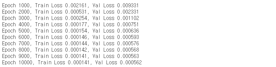
5. 학습시키기

5-1. MLE 모델

epochs = 10000
print_ = 1000
optim = torch.optim.Adam(mle_model.parameters())

train(model=mle_model,
      loss_fn=MSE,
      n_epoch=epochs,
      opt=optim,
      x_train=x_train,y_train=y_train,
      x_val=x_val,y_val=y_val,
      print_=print_,type=1)

with torch.no_grad():
  Y_mle_pred = mle_model(X)

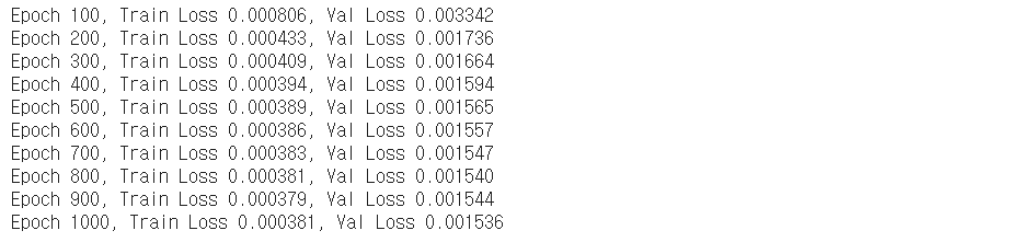
5-2. Variational Regression 모델

epochs = 1000
print_ = 100
optim = torch.optim.Adam(vi_model.parameters())

train(model=vi_model,
      loss_fn=neg_ELBO,
      n_epoch=epochs,
      opt=optim,
      x_train=x_train,y_train=y_train,
      x_val=x_val,y_val=y_val,
      print_=print_,type=2)

Variational Regression의 ouptut값은 deterministic하지 않다.

이를(feed forward) 1000번 반복하여, 각 data당 1000개의 결과값을 출력하여 저장한다.

with torch.no_grad():
  Y_vi_pred = torch.cat([vi_model(X)[0] for _ in range(1000)], dim=1)

6. Visualization

( xxx.detach().cpu()를 통해 다시 cpu에서 흐르게끔 바꾼 뒤 시각화를 해줘야 한다 )

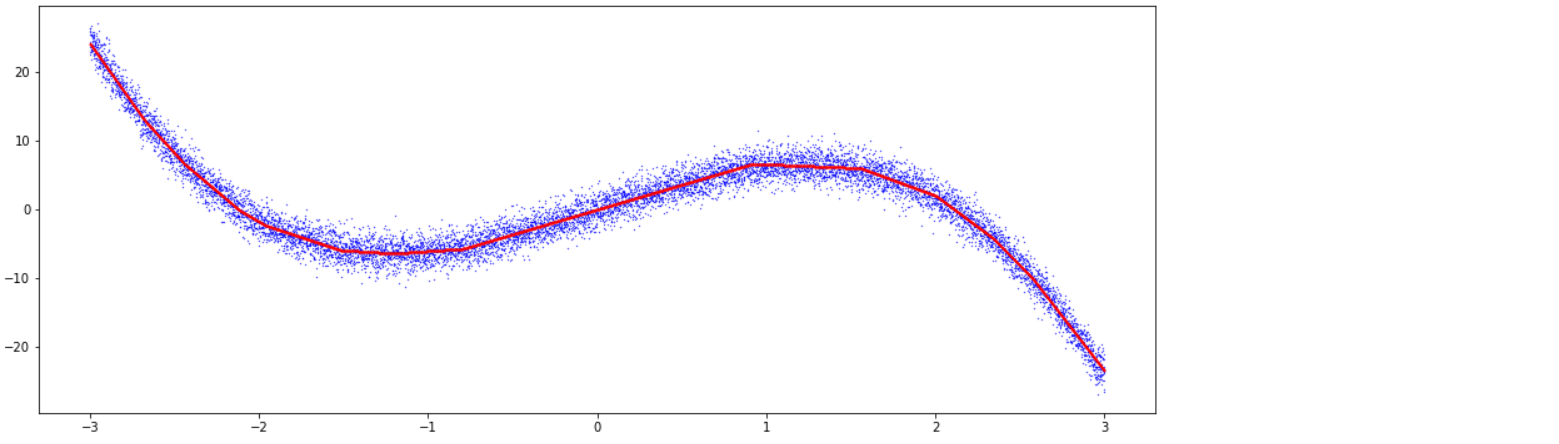
6-1. MLE 모델

plt.figure(figsize=(16, 6))
plt.scatter(X.detach().cpu(), Y_noise.detach().cpu(),color='blue',s=0.1)
plt.scatter(X.detach().cpu(), Y_mle_pred.detach().cpu(),color='red',s=0.1)
#plt.plot(X, mu)
#plt.fill_between(X.detach().cpu().flatten(), q1, q2, alpha=0.2)

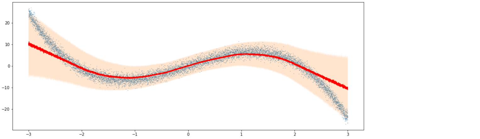
6-2. Variational Regression 모델

q1, mu, q2 = np.quantile(Y_vi_pred.detach().cpu(), [0.05, 0.5, 0.95], axis=1)

plt.figure(figsize=(16, 6))
plt.scatter(X.detach().cpu(), Y_noise.detach().cpu(),s=0.1)
plt.plot(X.detach().cpu(), mu,color='red')
plt.fill_between(X.detach().cpu().flatten(), q1, q2, alpha=0.2)

Twitter Facebook LinkedIn

(Pytorch) 02.Variational Inference

Seunghan Lee

Variational Inference

1. Import Packages

2. 가상 데이터 생성

3. Train 함수

4. Model & Loss Function 구현

4-1. MLE

(1) Model

(2) Loss Function

4-2. Variational Regression

(1) Model

(2) Loss Function

5. 학습시키기

5-1. MLE 모델

5-2. Variational Regression 모델

6. Visualization

6-1. MLE 모델

6-2. Variational Regression 모델

You May Also Enjoy