
( Skip the basic parts + not important contents )
8. Graphical Models
Advantageous to use “diagrammatic representations”
\(\rightarrow\) called “PGM” (Probabilistic Graphical Models)
Main useful properties of PGM
- 1) simple way to visualize the ‘structure of probabilistic model’
- 2) insights, such as conditional independence can be obtained by seeing the graph
- 3) complex computations can be expressed graphically
Concepts
- nodes (vertices) : random variable
- links (edges, arcs) : probabilistic relations between variables
- parent node / child node
\(\rightarrow\) captures “joint pdf” over all r.v, which can be decomposed into a product of factors
Will talk about
- “Bayesian Network” ( = Directed graphical models )
- “Markov Random Fields” ( = Undirected graphical models )
Convenient to convert both types of graphs into a representation, called “factor graph”
8-1. Bayesian Networks
( = Directed graphical models )
Product rule
- \(p(a, b, c)=p(c \mid a, b) p(a, b)\).
- \(p(a, b, c)=p(c \mid a, b) p(b \mid a) p(a)\).
- left ) symmetrical
- right ) not symmetrical
Joint pdf of K variables :
-
\(p\left(x_{1}, \ldots, x_{K}\right)=p\left(x_{K} \mid x_{1}, \ldots, x_{K-1}\right) \ldots p\left(x_{2} \mid x_{1}\right) p\left(x_{1}\right)\).
-
Fully connected = link between every pair of nodes
-
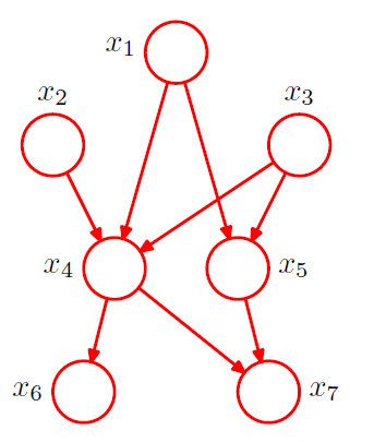
Not Fully connected : absence of links! convey interesting informations
ex) \(p\left(x_{1}\right) p\left(x_{2}\right) p\left(x_{3}\right) p\left(x_{4} \mid x_{1}, x_{2}, x_{3}\right) p\left(x_{5} \mid x_{1}, x_{3}\right) p\left(x_{6} \mid x_{4}\right) p\left(x_{7} \mid x_{4}, x_{5}\right)\)
General expression of graph with K nodes
-
joint pdf : \(p(\mathbf{x})=\prod_{k=1}^{K} p\left(x_{k} \mid \mathrm{pa}_{k}\right)\)
where \(\text{pa}_k\) : a set of parents of \(x_k\)
DAGS ( = Directed Acyclic graphs )
-
no directed cycles
( = no closed paths within the graph, such that we can move from node to node along links following the direction of the arrows and end up back at the starting node )
8-1-1. Example : Polynomial Regression
( Bayesian polynomial regression )
Joint pdf = prior \(p(w)\) \(\times\) \(N\) conditional distn \(p(t_n\mid w)\)
- \(p(\mathbf{t}, \mathbf{w})=p(\mathbf{w}) \prod_{n=1}^{N} p\left(t_{n} \mid \mathbf{w}\right)\).
More complex models
-
inconvenient to write out all the nodes from \(t_1\) .. .\(t_N\)
\(\rightarrow\) use “plate”
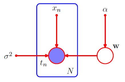
Plate
-
labeled with \(N\) ( = N nodes )
-
open circles = random variables
-
solid circles = deterministic parameters
-
ex) \(p\left(\mathbf{t}, \mathbf{w} \mid \mathbf{x}, \alpha, \sigma^{2}\right)=p(\mathbf{w} \mid \alpha) \prod_{n=1}^{N} p\left(t_{n} \mid \mathbf{w}, x_{n}, \sigma^{2}\right)\)
- \(\{t_n\}\) : observed variables / shaded
- \(w\) : not observed ( = latent variables / hidden variables ) / not shaded
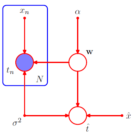
We are not interested in \(w\), but instead “predictions of new input variables”
- \(p\left(\widehat{t}, \mathbf{t}, \mathbf{w} \mid \widehat{x}, \mathbf{x}, \alpha, \sigma^{2}\right)=\left[\prod_{n=1}^{N} p\left(t_{n} \mid x_{n}, \mathbf{w}, \sigma^{2}\right)\right] p(\mathbf{w} \mid \alpha) p\left(\widehat{t} \mid \widehat{x}, \mathbf{w}, \sigma^{2}\right)\).
8-1-2. Generative Models
wish to draw samples from given pdf : “ancestral sampling”
Goal : draw a sample \(\hat{x_1},....,\hat{x_K}\)
Assumption
-
variables have been ordered
-
no links from any node to any lower numbered node
( = each node has high number than their parents)
to sample from Marginal distribution …
- take the sampled values for the required nodes
- discard the remaining nodes
Typically…
-
high numbered variables : terminal nodes = represent “observation”
-
low numbered variables : “latent variables”
role of latent variables : make “complicated distribution” into “simpler”
Graphical model captures “causal process”
-
“how the data was generated”
-
called “Generative models”
\(\leftrightarrow\) Polynomial Regression model : not generative
\(\because\) no pdf associated with the input variable \(x\)
8-1-3. Discrete Variables
\(p(x\mid \mu)\) for a single discrete variable \(x\), having \(K\) classes
\[p(\mathbf{x} \mid \boldsymbol{\mu})=\prod_{k=1}^{K} \mu_{k}^{x_{k}}\]- \(\mu=\left(\mu_{1}, \ldots, \mu_{K}\right)^{\mathrm{T}}\).
- \(\sum_{k} \mu_{k}=1\).
- only \(K-1\) values for \(\mu_{k}\) needed
\(p(x_1,x_2\mid \mu)\) for a two discrete variable \(x\), each having \(K\) classes
\[p\left(\mathbf{x}_{1}, \mathbf{x}_{2} \mid \boldsymbol{\mu}\right)=\prod_{k=1}^{K} \prod_{l=1}^{K} \mu_{k l}^{x_{1 k} x_{2 l}}\]-
probability of observing both \(x_{1 k}=1\) and \(x_{2 l}=1\) by the parameter \(\mu_{k l}\)
( \(x_{1 k}\) denotes the \(k^{\text {th }}\) component of \(\mathrm{x}_{1}\), and similarly for \(x_{2 l}\) )
-
\(\sum_{k} \sum_{l} \mu_{k l}=1\).
-
only \(K^2-1\) values for \(\mu_{kl}\) needed
\(\rightarrow\) with \(M\) discrete variables, \(K^{M}-1\) needed
Using graphical methods in \(p(x_1,x_2\mid \mu)\)
-
product rule : \(p\left(\mathrm{x}_{1}, \mathrm{x}_{2}\right)\) = \(p\left(\mathrm{x}_{2} \mid \mathrm{x}_{1}\right) p\left(\mathrm{x}_{1}\right)\)
-
two node graph
-
link going from \(x_1\) to \(x_2\)
-
marginal \(p\left(\mathrm{x}_{1}\right)\) : \(K-1\) parameters
-
conditional \(p\left(\mathrm{x}_{2} \mid \mathrm{x}_{1}\right)\) : \(K-1\) parameters for each of the \(K\) possible values of \(\mathrm{x}_{1} .\)
\(\leftrightarrow\) \((K-1)+K(K-1)=K^{2}-1\).
-
Reducing the number of parameters
- (1) independence
- (2) chain of nodes
- (3) sharing parameters
- (4) Bayesian Modeling using prior
- (5) Parameterized models
(1) Independence between \(x_1\) and \(x_2\)
-
each is described by “separate” multinomial distribution
\(\rightarrow\) total number of parameters : \(2(K-1)\)
-
expand it to \(M\) independent random variables : \(M(K-1)\)
( if fully connected : \(K^M-1\) parameters )
-
but restricting the class of distribution!
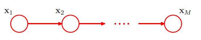
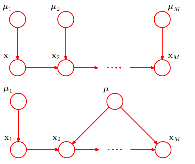
(2) Chain of nodes
-
\(p(x_1)\) : \(K-1\) parameters
-
\(p(x_i \mid x_{i-1})\) : \(M-1\) conditional distributions \(\times\) \(K(K-1)\) parameters
\(\rightarrow\) \(K-1 + (M-1)K(K-1)\) parameters
(3) Sharing parameters ( = tying of parameters)
-
in (2) Chain of nodes : \(K-1 + (M-1)K(K-1)\)
if conditional distributions share parameters : \(K-1 + K(K-1)\)
(4) Bayesian Modeling using prior
-
extension of (2)
-
use Dirichlet prior
( tied & untied )
(5) Parameterized Models
-
all of the nodes represent binary variables
( each of the parent variables \(x_i\) is governed by a single parameter \(\mu_i\) ( = \(p(x_i=1)\) ) )
-
would require \(2^M\) parameters!
( exponentially grow with \(M\) )
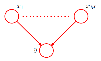
-
to reduce parameter, use “more parsimonious form” for conditional distribution,
using a “logistic sigmoid function” ( acting on a linear combination of parent variables )
\[p\left(y=1 \mid x_{1}, \ldots, x_{M}\right)=\sigma\left(w_{0}+\sum_{i=1}^{M} w_{i} x_{i}\right)=\sigma\left(\mathbf{w}^{\mathrm{T}} \mathbf{x}\right)\]where \(\mathbf{w}=\left(w_{0}, w_{1}, \ldots, w_{M}\right)^{\mathrm{T}}\) ( need only \(M+1\) parameters )
-
more restricted form, but number of parameter grows linearly!
-
analogous to the choice of restrictive form in covariance matrix in MVN
8-1-4. Linear-Gaussian models
MVN can be expressed as a directed graph!
-
allows us to impose interesting structure on the distribution
-
ex) linear-Gaussian models ( such as probabilistic PCA, FA, … )
\(D\) variables, where node \(i\) represents single continuous r.v. \(x_i\) having Gaussian distn
-
\(p\left(x_{i} \mid \mathrm{pa}_{i}\right)=\mathcal{N}\left(x_{i} \mid \sum_{j \in \mathrm{pa}_{i}} w_{i j} x_{j}+b_{i}, v_{i}\right)\).
-
log joint pdf : ( = log of the product of these conditionals )
\[\begin{aligned} \ln p(\mathrm{x}) &=\sum_{i=1}^{D} \ln p\left(x_{i} \mid \mathrm{pa}_{i}\right) \\ &=-\sum_{i=1}^{D} \frac{1}{2 v_{i}}\left(x_{i}-\sum_{j \in \mathrm{pa}_{i}} w_{i j} x_{j}-b_{i}\right)^{2}+\mathrm{cor} \end{aligned}\]( quadratic function of the components of \(x\) \(\rightarrow\) joint pdf \(p(x)\) is MVN )
Can find mean & covariance recursively!
( starting from the lowest numbered node )
\[x_{i}=\sum_{j \in \mathrm{pa}_{i}} w_{i j} x_{j}+b_{i}+\sqrt{v_{i}} \epsilon_{i}\]- \(\epsilon_{i} \sim N(0,I)\) & \(\mathbb{E}\left[\epsilon_{i} \epsilon_{j}\right]=I_{i j}\).
Mean and Covariance
\(\mathbb{E}\left[x_{i}\right]=\sum_{j \in \mathrm{pa}_{i}} w_{i j} \mathbb{E}\left[x_{j}\right]+b_{i}\).
( where \(\mathbb{E}[\mathrm{x}]=\left(\mathbb{E}\left[x_{1}\right], \ldots, \mathbb{E}\left[x_{D}\right]\right)^{\mathrm{T}}\) )
\(\begin{aligned} \operatorname{cov}\left[x_{i}, x_{j}\right] &=\mathbb{E}\left[\left(x_{i}-\mathbb{E}\left[x_{i}\right]\right)\left(x_{j}-\mathbb{E}\left[x_{j}\right]\right)\right] \\ &=\mathbb{E}\left[\left(x_{i}-\mathbb{E}\left[x_{i}\right]\right)\left\{\sum_{k \in \mathrm{pa}_{j}} w_{j k}\left(x_{k}-\mathbb{E}\left[x_{k}\right]\right)+\sqrt{v_{j}} \epsilon_{j}\right\}\right] \\ &=\sum_{k \in \mathrm{pa}_{j}} w_{j k} \operatorname{cov}\left[x_{i}, x_{k}\right]+I_{i j} v_{j} \end{aligned}\).
2 extreme cases
- 1) no links
- 2) fully connected
1) No links
- \(D\) isolated nodes
- no parameters \(w_{ij}\)
- \(2D\) parameters
- \(b_i\) : \(D\).
- \(v_i\) : \(D\).
- mean of \(p(x)\) : \(\left(b_{1}, \ldots, b_{D}\right)^{\mathrm{T}}\)
- covariance of \(p(x)\) : \(\operatorname{diag}\left(v_{1}, \ldots, v_{D}\right)\)
2) Fully connected
- \(D(D+1)/2\) parameters
- \((D^2-D)/2\) : \(w_{ij}\) where \(i\neq j\) & elements only below the diagonal
- \(D\) : diagonal
3) Intermediate
-
example)
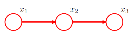
-
mean and covariance :
\(\begin{aligned} \boldsymbol{\mu} &=\left(b_{1}, b_{2}+w_{21} b_{1}, b_{3}+w_{32} b_{2}+w_{32} w_{21} b_{1}\right)^{\mathrm{T}} \\ \boldsymbol{\Sigma} &=\left(\begin{array}{cc} v_{1} & w_{21} v_{1} & w_{32} w_{21} v_{1} \\ w_{21} v_{1} & v_{2}+w_{21}^{2} v_{1} & w_{32}\left(v_{2}+w_{21}^{2} v_{1}\right) \\ w_{32} w_{21} v_{1} & w_{32}\left(v_{2}+w_{21}^{2} v_{1}\right) & v_{3}+w_{32}^{2}\left(v_{2}+w_{21}^{2} v_{1}\right) \end{array}\right) \end{aligned}\).
-
conditional distribution for node \(i\)
\(p\left(\mathbf{x}_{i} \mid \mathrm{pa}_{i}\right)=\mathcal{N}\left(\mathbf{x}_{i} \mid \sum_{j \in \mathrm{pa}_{i}} \mathbf{W}_{i j} \mathbf{x}_{j}+\mathbf{b}_{i}, \mathbf{\Sigma}_{i}\right)\).
We have seen a case of “conjugate prior” ( all Gaussians )
can also use hyperparameter
- hyperprior : prior over the hyperparameter
- can again treat it from a Bayesian persepective
- further, “hierarchical Bayesian model”
8-2. Conditional Independence
\[\begin{aligned} p(a, b \mid c) &=p(a \mid b, c) p(b \mid c) \\ &=p(a \mid c) p(b \mid c) \end{aligned}\] \[a \perp b \mid c\]8-2-1. three examples
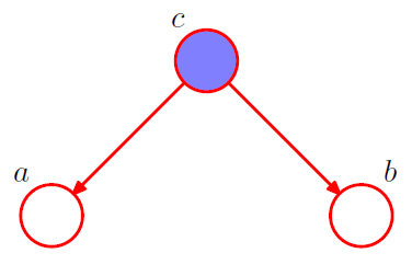
[ example 1 ] Diverging Connections
1-1. \(p(a, b, c)=p(a \mid c) p(b \mid c) p(c)\).
Is \(a\) and \(b\) independent ?
-
\(p(a, b)=\sum_{c} p(a \mid c) p(b \mid c) p(c)\).
\(\rightarrow\) No! \(a \not \perp b \mid \emptyset\).
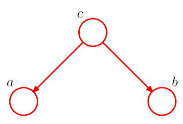
1-2. condition on \(c\) from 1-1
\[\begin{aligned} p(a, b \mid c) &=\frac{p(a, b, c)}{p(c)} \\ &=p(a \mid c) p(b \mid c) \end{aligned}\]\(\rightarrow\) YES! \(a \perp b \mid c\)
-
node \(c\) : “tail-to-tail”
( \(\because\) node is connected to the tails of the two arrows )
-
node \(c\) blocks the path from \(a\) to \(b\) \(\rightarrow\) cause them to be (conditionally) independent
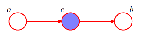
[ example 2 ] Serial Connections
2-1. \(p(a, b, c)=p(a) p(c \mid a) p(b \mid c)\).
Is \(a\) and \(b\) independent ?
-
\(p(a, b)=p(a) \sum_{c} p(c \mid a) p(b \mid c)=p(a) p(b \mid a)\).
\(\rightarrow\) No! \(a \not \perp b \mid \emptyset\).
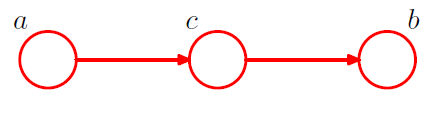
2-2. condition on \(c\) from 2-1
\(\begin{aligned} p(a, b \mid c) &=\frac{p(a, b, c)}{p(c)} \\ &=\frac{p(a) p(c \mid a) p(b \mid c)}{p(c)} \\ &=p(a \mid c) p(b \mid c) \end{aligned}\).
\(\rightarrow\) YES! \(a \perp b \mid c\)
- node \(c\) : “head-to-tail”
- node \(c\) blocks the path from \(a\) to \(b\) \(\rightarrow\) cause them to be (conditionally) independent
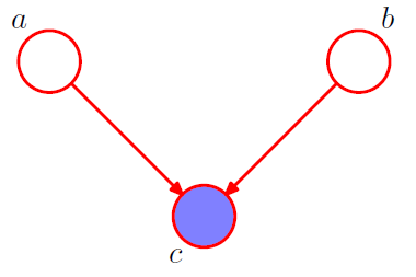
[ example 3 ] Converging Connections
3-1. \(p(a, b, c)=p(a) p(b) p(c \mid a, b)\).
Is \(a\) and \(b\) independent ?
-
\(p(a, b)=p(a) p(b)\).
\(\rightarrow\) Yes! \(a \perp b \mid \emptyset\).
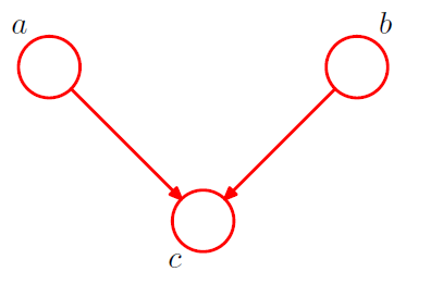
3-2. condition on \(c\) from 3-1
\(\begin{aligned} p(a, b \mid c) &=\frac{p(a, b, c)}{p(c)} \\ &=\frac{p(a) p(b) p(c \mid a, b)}{p(c)} \end{aligned}\).
\(\rightarrow\) NO! \(a \not \perp b \mid c\)
-
node \(c\) : “head-to-head”
( \(\because\) node is connected to the heads of the two arrows )
-
when \(c\) is unobserved, it blocks the path
however, conditioning on \(c\) unblocks the path, and make them dependent!
8-2-2. D-separation
not finished
8-3. Markov Random Fields
not finished