( 참고 : https://www.youtube.com/watch?v=0yzwg9e3fbs )
Representation Learning
Raw feature space에서, 보다 유의미한 latent space로 매핑시키자!
Representation Learning = Feature Learning
Self-supervised Contrastive Learning
Self-supervised Learning
- Labeled된 데이터가 부족한 상황에서 주로 사용
세 종류의 데이터
- Anchor : 학습 대상의 데이터
- Positive : 증강 데이터
- Negative : 나머지 데이터
목표 :
- anchor & positive은 유사하도록
- anchor & negative는 상이하도록
\(L=\sum_{i \in I} L_{i}^{\text {self }}=-\sum_{i \in I} \log \frac{\exp \left(\mathbf{z}_{\boldsymbol{i}} \cdot \mathbf{z}_{\boldsymbol{j}(i)} / \tau\right)}{\sum_{a \in A(i)} \exp \left(\mathbf{z}_{\boldsymbol{i}} \cdot \mathbf{z}_{\boldsymbol{a}} / \tau\right)}\).
- \(i\) : 학습 대상 데이터( Anchor )의 index
- \(i \in \{1, \cdots 2N\}\) .
- \(N\) 개 : 학습 데이터
- \(N\)개 : 증강 데이터
- \(i \in \{1, \cdots 2N\}\) .
- \(j(i)\) : Positive 데이터 ( = Anchor \(i\)를 증강한 데이터 )
- \(k \in A(i) \text{\\} \{j(i)\}\) : Negative 데이터 ( \(2N-2\) 개 )
- 전체 (2N) - Anchor & Positive (2)
- \(a \in A(i)\) : Anchor \(i\) 외의 나머지 데이터 ( \(2N -1\) 개 )
- 전체 (2N) - Anchor (1)
학습 방향
- 분자는 maximize
- \(\exp \left(\mathbf{z}_{\boldsymbol{i}} \cdot \mathbf{z}_{\boldsymbol{j}(i)} / \tau\right)\).
- 유사한건 가깝도록
- 분모는 minimize
- \(\sum_{a \in A(i)} \exp \left(\mathbf{z}_{\boldsymbol{i}} \cdot \mathbf{z}_{\boldsymbol{a}} / \tau\right)\).
- 상이한건 멀도록
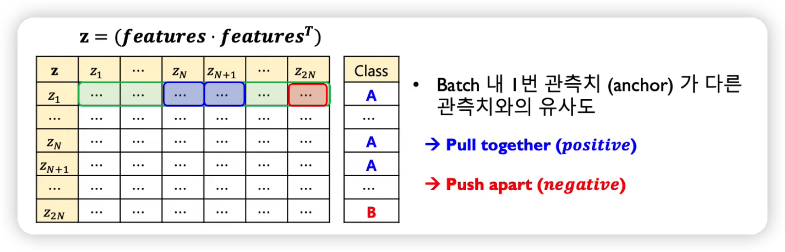
BUT… 같은 y label이 달린 데이터도, negative에 속할 경우 상이하도록 학습이 유도된다는 점!
\(\rightarrow\) Supervised Contrastive Learning의 등장
Supervised Contrastive Learning
(1) Supervised Learning
(2) Self-Supervised Contrastive Learning
이 두가지의 장점을 활용!
-
정답(y-label)이 같은 것은 가깝도록
-
정답(y-label)이 다른 것은 멀도록
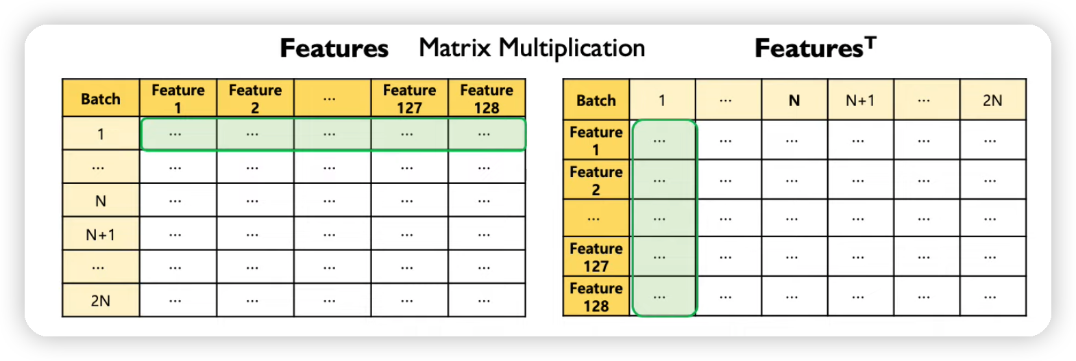
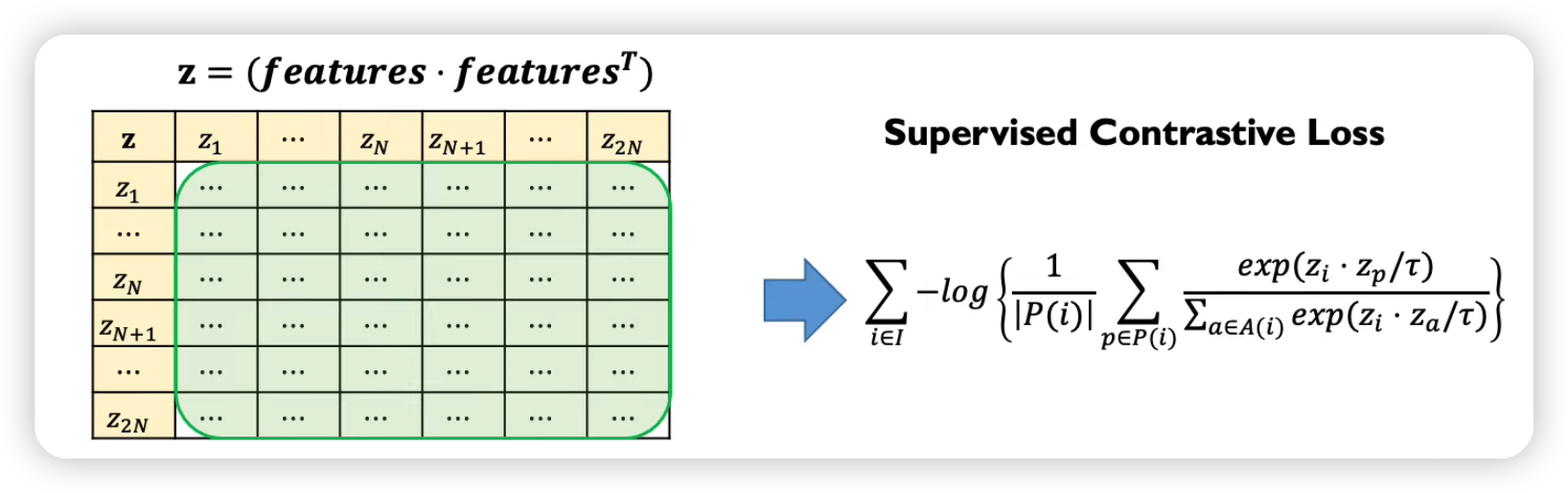
\(L=\sum_{i \in I} L_{i}^{s u p}=\sum_{i \in I}-\log \left\{\frac{1}{ \mid P(i) \mid } \sum_{p \in P(i)} \frac{\exp \left(z_{i} \cdot z_{p} / \tau\right)}{\sum_{a \in A(i)} \exp \left(z_{i} \cdot z_{a} / \tau\right)}\right\}\).
-
\(\frac{1}{ \mid P(i) \mid } \sum_{p \in P(i)}\) term이 추가된 것을 확인할 수 있다.
- notation은 위와 동일
- 추가
- \(P(i) \equiv\left\{p \in A(i): \tilde{y}_{p}=\tilde{y}_{i}\right\}\) = set of indices of all positive samples
- 비교하기
- self-supervised : positive sample이 1개
- supervised : positive sample이 여러 개 ( 같은 label은 전부 positive )
- \(a \in A(i) \equiv I \backslash\{i\}\) { (anchor 외 모든 데이터 }
- \(\mid P(i ) \mid\) 개 positives
- \(2 \mathrm{~N} - \mid P(i) \mid\) 개 negatives
Steps
step 1) pre-training
- (1) augmentation
- (2) encoder
- (3) projection head
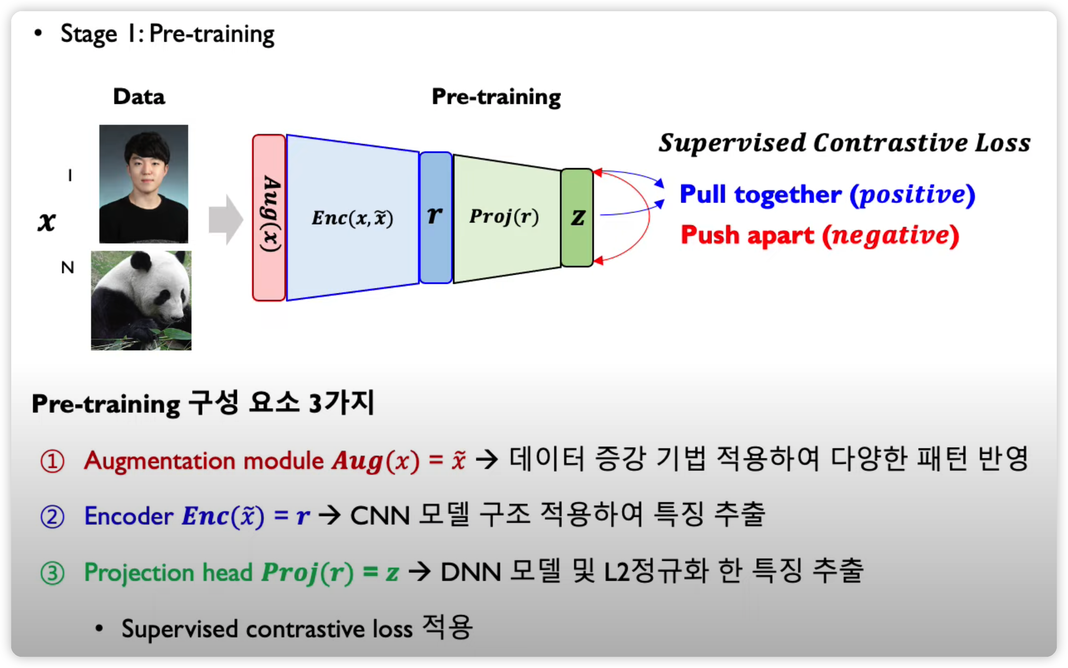
(1) Augmentation
-
crop, resize, distort , rotate, cutout ….
-
매 학습마다 random하게 augmentation
( + 여러 개 동시에 적용 가능 )
(2) Encoder
- CNN으로 feature extraction 한 뒤, GAP 등으로 특징 벡터 추출
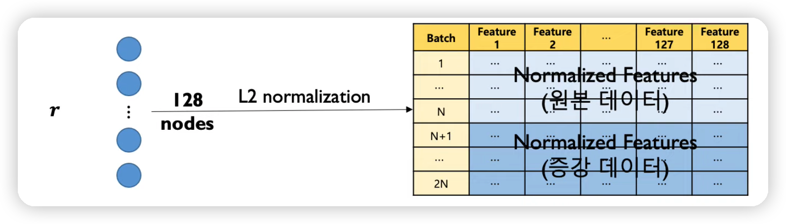
(3) Projection Head
- loss를 적용할 space로 매핑