(paper) Balanced Graph Structure Learning for MTS Forecasting

Balanced Graph Structure Learning for MTS Forecasting (2022)

Contents

1. Abstract
2. Introduction
3. Graph Structure Learning
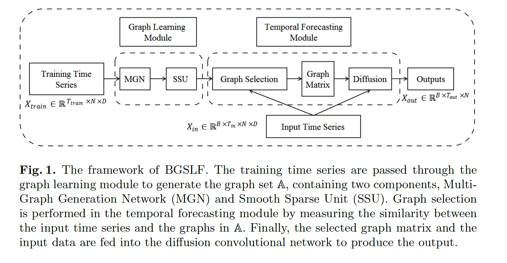
4. Methodology
   1. Graph Structure Learning module
      1. MGN
      2. SSU
   2. Temporal Forecasting module
      1. Graph Selection
      2. DCRNN

0. Abstract

Propose

• without the need of pre-defined graphs

• balance the trade-off between efficiency & flexibility

BGSLF (Baalnced Graph Structure Learning for MTS Forecasting)

Modules

• (1) MGN (Multi-Graph Generation Network)
• (2) Graph Selection Module
  • (1) & (2) \(\rightarrow\) to balance the trade-off
• (3) SSU (Smooth Sparse Unit)
  • to design sparse graph structure

1. Introduction

Contributions

1. Propose BGSLF

   • aim of learning smooth & sparse dependencies between variables
   • can generate a specified number of graphs
   • then, can select BEST graph per input

2. Graph Structure Learning module

   • incorporate domain knowledge

     \(\rightarrow\) save lots of parameters

3. SSU (Smooth Sparse Unit)

   • to infer continuous & sparse dependencies
   • no need of non-differentiable functions
     • ex) Top-K, Regularization

2. Graph Stucture Learning

Recent works

• consider spatial & temporal SEPERATELY

GWN (Graph Wave Net)

• use adaptive \(A\)

STAWnet

• attention to get self-learned node embedding

  ( to capture spatial embedding )

GWN & STAWnet : use Dilated Causal Convolution

MTGNN

• learn 2 embedding vectors per node
• then obtain \(A\)

GDN

• node embedding per node
• then build k\(NN\) graph

AGCRN

• 2 adaptive modules for enhancing GCN
• infer dynamic spatial relations

3. Methodology

(1) Graph Structure Learning module

a) MGN (Multi-Graph Generation Network)

• extract dynamic spatial relationships
• use difference operation

\(\begin{aligned} \operatorname{Diff}\left(\mathbf{X}_{:, 1}, \mathbf{X}_{i:, 2}, \mathbf{X}_{i, 3}, \cdots, \mathbf{X}_{i, T}\right) &=\left\{\mathbf{X}_{:, 2}-\mathbf{X}_{:, 1}, \mathbf{X}_{:, 3}-\mathbf{X}_{i, 2}, \cdots, \mathbf{X}_{i, T}-\mathbf{X}_{i, T-1}\right\} \\ & \triangleq\left\{\hat{\mathbf{X}}_{:, 1}, \hat{\mathbf{X}}_{i, 2}, \ldots, \hat{\mathbf{X}}_{:, T-1}\right\} \end{aligned}\).

Considering periodicity of TS, set period \(P\) to segment MTS

\(\rightarrow\) \(S=\left\lfloor T_{\text {train }} / P\right\rfloor\)

• then, concatenate them!
• \(\mathcal{O}=\left[\hat{\mathbf{X}}_{\mathbf{1}}, \hat{\mathbf{X}}_{\mathbf{2}} \ldots \ldots \hat{\mathbf{X}}_{\mathbf{S}}\right] \in \mathbb{R}^{S} \times N \times D \times P\).

Then, use 2d-conv & FC layer to obtain \(R\) graphs

\(\rightarrow\) These constitute the graph set \(\mathbb{A}\).

b) SSU (Smooth Sparse Unit)

• to learn continuous & sparse graphs

2 function : \(f\) & \(\varphi\)

• [smooth function 1] \(f: \mathbb{R} \rightarrow \mathbb{R}\)
  • \(f(x)= \begin{cases}e^{-\frac{1}{x}} & (x>0) \\ 0 & (x \leq 0)\end{cases}\).
• [smooth function 2] \(\varphi: \mathbb{R} \rightarrow[0,1]\)
  • \(\varphi(x)=\frac{\alpha f(x)}{\alpha f(x)+f(1-x)}\left(\alpha \in \mathbb{R}_{+}\right)\).
    • \(\varphi(x) \equiv\) 0 for \(x \leq 0\)
    • \(\varphi(x) \in(0,1)\) for \(0<x<1\)
    • \(\varphi(x) \equiv 1\) for \(x \geq 1\).

Output adjacency matrix : \(A=\frac{\alpha f(G)}{\alpha f(G)+f(\mathbf{1}-G)}\)

• \(G \in \mathbb{R}^{N \times N}\) : output of FC layer in (a)

(2) Temporal Forecasting module

a) Graph Selection

• from \(R\) graphs, select the best one ( finding optimal graph structure )
• for each TS \(X_{\text {in }} \in \mathbb{R}^{B \times T_{\mathrm{in}} \times N \times D}\),
  • select the best graph!

Optimal graph : \(A=\underset{A_{i} \in \mathbb{A}}{\arg \max } \cos \left\langle\mathcal{X}^{T} \mathcal{X}, A_{i}\right\rangle\)

• \(\cos \langle\mathcal{X}, \mathcal{Y}\rangle=\frac{\sum_{i, j} x_{i j} y_{i j}}{\sqrt{\sum_{i, j} x_{i j}^{2} \cdot \sum_{i, j} y_{i j}^{2}}}\),
• \(\mathcal{X}=\sum_{i=1}^{B} \sum_{j=1}^{D} X_{\text {in }[i,:,:, j]} \in \mathbb{R}^{T_{\mathrm{in}} \times N}\),