(paper 10) Your Contrastive Learning is Secretly Doing Stochastic Neighbor Embedding

Your Contrastive Learning is Secretly Doing Stochastic Neighbor Embedding

Contents

1. Abstract
2. Introduction
3. Preliminary & Related Work
   1. Notations
   2. SNE (Stochastic neighbor embedding)
   3. SSCL (Self-supervised contrastive learning)
4. SNE perspective of SSCL
   1. Analysis

0. Abstract

SSCL (Self-Supervised Contrastive Learning)

• extract powerful features from UN-labeled data

This paper :

• unconver connection between SSCL & SNE

In the persepective of SNE…

• (goal of SNE) match pairwise distance
• SSCL = special case with the input space pairwise distance specified by constructed “postive pairs” from data augmentation

1. Introduction

SSCL : updated by encouraging …

• the positive pairs close to each other

• the negative pairs away

BUT…theoretical understadning is under-explored

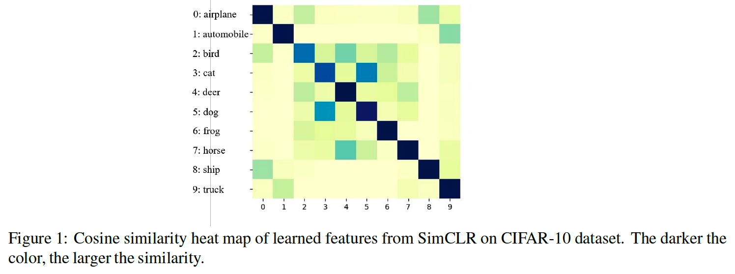
[ Similarity Heatmap of features learned by SimCLR ]

Contributions

• (1) propose a novel perspective that interprets SSCL methods as a type of SNE methods,

  with the aim of preserving pairwise similarities specified by the data augmentation.

• (2) provide novel theoretical insgihts for domain-agnostic data augmentation & implicit biases

  • 2-1) Isotropic random noise augmentations : induces \(l_2\) similarity
  • 2-2) Mixup noise : adapt to low-dim structures of data

• (3) propose several modifications to existing SSCL methods

2. Preliminary & Related Work

(1) Notations

For a function \(f: \Omega \rightarrow \mathbb{R}\) ….

• \(\mid \mid f \mid \mid _{\infty}=\sup _{\boldsymbol{x} \in \Omega} \mid f(\boldsymbol{x}) \mid\).
• \(\mid \mid f \mid \mid _{p}=\left(\int_{\Omega} \mid f(\boldsymbol{x}) \mid ^{p} d \boldsymbol{x}\right)^{1 / p}\).

For a vector \(\boldsymbol{x}\) …

• \(\mid \mid \boldsymbol{x} \mid \mid _{p}\) = \(p\)-norm

Norm

• function norms : \(L_{p}\)
• vector norms : \(l_{p}\)

Probability

• \(\mathbb{P}(A)\) : probability of event \(A\)
• \(P_{z}\) : probability distribution
• \(p_z\) : density

Datasets : \(\mathcal{D}_{n}=\left\{\boldsymbol{x}_{1}, \cdots, \boldsymbol{x}_{n}\right\} \subset \mathbb{R}^{d}\)

• each \(\boldsymbol{x}_{i}\) independently follows distribution \(P_{\boldsymbol{x}}\)

• low dim version : \(\boldsymbol{z}_{1}, \cdots, \boldsymbol{z}_{n} \in \mathbb{R}^{d_{z}}\)

  ( goal : find informative low-dimensional features \(\boldsymbol{z}_{1}, \cdots, \boldsymbol{z}_{n} \in \mathbb{R}^{d_{z}}\) of \(\mathcal{D}_{n}\) )

Feature Mapping : \(f(\boldsymbol{x})\)

• from \(\mathbb{R}^{d} \rightarrow \mathbb{R}^{d_{z}}\), i.e., \(\boldsymbol{z}_{i}=f\left(\boldsymbol{x}_{i}\right)\)

(2) SNE (Stochastic neighbor embedding)

Goal :

• map high-dim to low-dim, while preserving as much neighboring information as possible

Neighboring information :

• captured by pairwise relationships

Training process :

• step 1) DATA space
  • calculate the pairwise similarity matrix \(\boldsymbol{P} \in \mathbb{R}^{n \times n}\) for \(\mathcal{D}_{n}\)
• step 2) FEATURE space
  • optimize features \(\boldsymbol{z}_{1}, \cdots, \boldsymbol{z}_{n}\) such that their pairwise similarity matrix \(\boldsymbol{Q} \in \mathbb{R}^{n \times n}\) matches \(\boldsymbol{P}\).

(Hinton and Roweis, 2002)

• pairwise similarity = conditional probabilities of \(\boldsymbol{x}_{j}\) being the neighbor of \(\boldsymbol{x}_{i}\)

  ( induced by a Gaussian distribution centered at \(\boldsymbol{x}_{i}\), i.e., when \(i \neq j\) )

• DATA space : \(P_{j \mid i}\)

  • \(P_{j \mid i}=\frac{\exp \left(-d\left(\boldsymbol{x}_{i}, \boldsymbol{x}_{j}\right)\right)}{\sum_{k \neq i} \exp \left(-d\left(\boldsymbol{x}_{i}, \boldsymbol{x}_{k}\right)\right)}\).

• FEATURE space : \(Q_{j \mid i}\)

KL-divergence between \(P\) & \(Q\)

( = overall training objective for SNE )

• \(\inf _{\boldsymbol{z}_{1}, \cdots, \boldsymbol{z}_{n}} \sum_{i=1}^{n} \sum_{j=1}^{n} P_{j \mid i} \log \frac{P_{j \mid i}}{Q_{j \mid i}}\).

Improvement : t-SNE

• modifications
  • (1) conditional dist \(\rightarrow\) joint distn
  • (2) Gaussian \(\rightarrow\) \(t\)-distn
• \(Q_{i j}=\frac{\left(1+ \mid \mid \boldsymbol{z}_{i}-\boldsymbol{z}_{j} \mid \mid _{2}^{2}\right)^{-1}}{\sum_{k \neq l}\left(1+ \mid \mid \boldsymbol{z}_{k}-\boldsymbol{z}_{l} \mid \mid _{2}^{2}\right)^{-1}}\).
• ( for more about t-SNE … https://seunghan96.github.io/ml/stat/t-SNE/ )

(3) SSCL (Self-supervised contrastive learning)

Key Part : construction of POSITIVE pairs

( = different views of same sample )

Data Augmentation : \(\boldsymbol{x}_{i}^{\prime}=t\left(\boldsymbol{x}_{i}\right)\)

Augmented Datasets : \(\mathcal{D}_{n}^{\prime}=\left\{\boldsymbol{x}_{1}^{\prime}, \cdots, \boldsymbol{x}_{n}^{\prime}\right\}\)

Loss Function : \(l\left(\boldsymbol{x}_{i}, \boldsymbol{x}_{i}^{\prime}\right)=-\log \frac{\exp \left(\operatorname{sim}\left(f\left(\boldsymbol{x}_{i}\right), f\left(\boldsymbol{x}_{i}^{\prime}\right)\right) / \tau\right)}{\sum_{x \in \mathcal{D}_{n} \cup \mathcal{D}_{n}^{\prime} \backslash\left\{\boldsymbol{x}_{i}\right\}} \exp \left(\operatorname{sim}\left(f\left(\boldsymbol{x}_{i}\right), f(\boldsymbol{x})\right) / \tau\right)}\).

• \(\operatorname{sim}\left(\boldsymbol{z}_{1}, \boldsymbol{z}_{2}\right)=\left\langle\frac{\boldsymbol{z}_{1}}{ \mid \mid \boldsymbol{z}_{1} \mid \mid _{2}}, \frac{\boldsymbol{z}_{2}}{ \mid \mid \boldsymbol{z}_{2} \mid \mid _{2}}\right\rangle\) .

InfoNCE : \(L_{\text {InfoNCE }}:= \frac{1}{2 n} \sum_{i=1}^{n}\left(l\left(\boldsymbol{x}_{i}, \boldsymbol{x}_{i}^{\prime}\right)+l\left(\boldsymbol{x}_{i}^{\prime}, \boldsymbol{x}_{i}\right)\right)\)

3. SNE perspective of SSCL

SimCLR = special SNE model

• datsaet : \(\widetilde{\mathcal{D}}_{2 n}=\mathcal{D}_{n} \cup \mathcal{D}_{n}^{\prime}\)
  • \(\widetilde{\boldsymbol{x}}_{2 i-1}=\boldsymbol{x}_{i}\) and \(\widetilde{\boldsymbol{x}}_{2 i}=\boldsymbol{x}_{i}^{\prime}\) for \(i \in[n]\).
• feature space of SimCLR : unit sphere \(\mathbb{S}^{d_{z}}\)
  • pairwise distance : cosine distance
    • \(d\left(\boldsymbol{z}_{1}, \boldsymbol{z}_{2}\right)=1-\operatorname{sim}\left(\boldsymbol{z}_{1}, \boldsymbol{z}_{2}\right)\).
• for \(i \neq j\) …
  • \(\widetilde{Q}_{j \mid i}=\frac{\exp \left(\operatorname{sim}\left(f\left(\widetilde{\boldsymbol{x}}_{i}\right), f\left(\widetilde{\boldsymbol{x}}_{j}\right)\right)\right.}{\sum_{k \neq i} \exp \left(\operatorname{sim}\left(f\left(\widetilde{\boldsymbol{x}}_{i}\right), f\left(\widetilde{\boldsymbol{x}}_{k}\right)\right)\right.}\)……. ( similarity in DATA space )

By taking

\(\widetilde{P}_{j \mid i}= \begin{cases}\frac{1}{2 n}, & \text { if } \widetilde{\boldsymbol{x}}_{i} \text { and } \widetilde{\boldsymbol{x}}_{i} \text { are positive pairs } \\ 0, & \text { otherwise }\end{cases}\)….. ( similarity in FEATURE space )

\(\begin{aligned} \sum_{i=1}^{2 n} \sum_{j=1}^{2 n} \widetilde{P}_{j \mid i} \log \frac{\widetilde{P}_{j \mid i}}{\widetilde{Q}_{j \mid i}} &=\sum_{k=1}^{n}\left(\widetilde{P}_{2 k-1 \mid 2 k} \log \frac{\widetilde{P}_{2 k-1 \mid 2 k}}{\widetilde{Q}_{2 k-1 \mid 2 k}}+\widetilde{P}_{2 k \mid 2 k-1} \log \frac{\widetilde{P}_{2 k \mid 2 k-1}}{\widetilde{Q}_{2 k \mid 2 k-1}}\right) \\ &=\frac{1}{2 n} \sum_{k=1}^{n}\left(-\log \left(\widetilde{Q}_{2 k-1 \mid 2 k}\right)-\log \left(\widetilde{Q}_{2 k \mid 2 k-1}\right)\right)+\log \left(\frac{1}{2 n}\right) \end{aligned}\).

• \(\widetilde{Q}_{2 k-1 \mid 2 k}=l\left(\boldsymbol{x}_{k}, \boldsymbol{x}_{k}^{\prime}\right)\).
• \(\widetilde{Q}_{2 k \mid 2 k-1}=l\left(\boldsymbol{x}_{k}^{\prime}, \boldsymbol{x}_{k}\right)\).

\(\rightarrow\) SNE objective (2.1) reduces to that of the SimCLR objective \(L_{\text {InfoNCE, }}\) ( up to a constant term only depending on \(n\) )

learning process of SSCL

also follows the two steps of SNE

• step 1) The positive pair construction specifies the similarity matrix \(\boldsymbol{P}\).
• step 2) The training process then matches \(\boldsymbol{Q}\) to \(\boldsymbol{P}\) by minimizing some divergence

SNE vs SSCL

\(P\) in SNE

• densely filled by \(l_p\) distance
• Ignores the semantic information within rich data like images and texts

\(P\) in SSCL

• omits all traditional distances in \(R_d\)

• only specifies semantic similarity through data augmentation

  \(\rightarrow\) \(P\) is sparsely filled only by positive pairs

(1) Analysis

feature learning process of SSCL

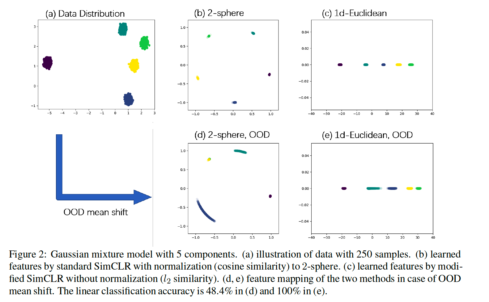
Toy dataset : Gaussian mixture setting

• \(P_{\boldsymbol{x}} \sim \frac{1}{m} \sum_{i=1}^{m} N\left(\boldsymbol{\mu}_{i}, \sigma^{2} \boldsymbol{I}_{d}\right)\).
  • ex) \(d=2, m=5, \sigma=0.1\) ……. 250 independent samples

a) Alignment & Uniformity

Perfect Alignment

• \(f\left(\boldsymbol{x}_{i}\right)=f\left(\boldsymbol{x}_{i}^{\prime}\right)\) for any \(i=1, \cdots, n\)

Perfect Uniformity

• if all pairs are maximally separated on the sphere
• Tammes problem
  • if \(d=2\) : mapped points form a regular polygon
  • if \(d \geq n-1\) : mapped points form a (n-1) simplex

By Figure 2-a) & 2-b)…

\(\rightarrow\) perfect alignment and perfect uniformity are almost achieved by standard SimCLR in the Gaussian mixture setting.

b) Domain-agnostic DA

(1) Random Noise Augmentation

\(\boldsymbol{x}^{\prime}=\boldsymbol{x}+\delta\), where \(\delta \sim \phi(\boldsymbol{x})\).

• pairwise similarity = \(P_{\boldsymbol{x}_{1}, \boldsymbol{x}_{2}}=\mathbb{P}\left(\boldsymbol{x}_{1}\right.\) and \(\boldsymbol{x}_{2}\) form a positive pair )

  • \(P_{\boldsymbol{x}_{1}, \boldsymbol{x}_{2}}=P_{\boldsymbol{x}_{2}, \boldsymbol{x}_{1}}=\phi\left(\boldsymbol{x}_{1}-\boldsymbol{x}_{2}\right)\).

• ex) noise distn = istoropic Gaussian

  \(\rightarrow\) distance is equivalent to \(l_2\) distance in \(R^d\)

(2) Mixup

convex combinations of the training data

\(\boldsymbol{x}_{i}^{\prime}=\boldsymbol{x}_{i}+\lambda\left(\boldsymbol{x}_{j}-\boldsymbol{x}_{i}\right)\) , where \(\lambda \in(0,1)\)

• convoluted density of \(\lambda\left(\boldsymbol{x}_{1}-\boldsymbol{x}_{2}\right)\) : \(p_{\lambda}(\boldsymbol{x})\)

• if employing mixup for positive pairs in SSCL

  \(\rightarrow\) \(P_{\boldsymbol{x}_{1}, \boldsymbol{x}_{2}}=P_{\boldsymbol{x}_{2}, \boldsymbol{x}_{1}}=p_{\lambda}\left(\boldsymbol{x}_{1}-\boldsymbol{x}_{2}\right)\)

Gaussian vs Mixup

• data-dependent mixup > Gaussian random noise

  ( from the perspective of “curse of dimensionality” )

• Setting :

  • \(d\)-dimensional Gaussian mixture setting with \(m<d\) separated components.
  • \(\boldsymbol{\mu}_{1}, \cdots, \boldsymbol{\mu}_{m}\) : can take up at most \((m-1)\)-dimensional linear sub-space of \(\mathbb{R}^{d}\)

[ Mixup ]

• ( for light-tailed Gaussian distribution )

  • majority of samples will be close to \(S_{\mu}\)
  • majority of the convoluted density \(p_{\lambda}(\boldsymbol{x})\) will also be supported on \(\boldsymbol{S}_{\mu}\)

  \(\rightarrow\) distance from mixup will omit irrelevant variations in the complement of \(S_{\mu}\)

  ( focus on low-dim subspace \(\boldsymbol{S}_{\mu}\) )

[ Gaussian Noise ]

• induces \(l_2\) distance for positive pairs with support of \(R^d\)

  \(\rightarrow\) much more inefficient

c) Implicit bias

xx