(paper 9) SwAV

Unsupervised Learning of Visual Features by Contrasting Cluster Assignments

Contents

1. Abstract
2. Introduction
3. Related Work
   1. Instance and Contrastive Learning
   2. Clustering for Deep Representation Learning
   3. Handcrafted pretext tasks
4. Method
   1. Online Clustering
   2. Multi-crop
5. Main Results
   1. Evaluating the unsupervised features on ImageNet
   2. Transferring unsupervised features to downstream tasks
   3. Training with small batches
6. Ablation Study

0. Abstract

Unsupervised Image Representations, via contrastive learning

• usually work online

• rely on large number of explicit pairwise feature comparison

  \(\rightarrow\) computationally challenging!

SwAV

• without requiring to compute pairwise comparison

• simultaneously clusters the data, while enforcing consistency between cluster assignments,

  produced for different augmentation of same image

  ( instead of comparing features directly )

• swapped prediction

  • predict the ”code” of a view from the ”representation” of another view

• memory efficient

  • does not require a large memory bank

multi-crop

• new data augmentation strategy
• mix of views with different resolutions

1. Introduction

Most of SOTA self-supervised learning

\(\rightarrow\) build upon the instance discrimination task

( each image = each class )

Instance Discrimination rely on combination of 2 elements

• (1) contrastive loss
• (2) set of image transformations

\(\rightarrow\) this paper improves both (1) & (2)

Contrastive Loss

• compares pairs of image representations
• BUT…computing pairwise \(\rightarrow\) not practical!

solutions to pairwise comparison ??

• (1) reduce the number of comparisons to random subsets of images

• (2) approximate the task

  • Ex) relax the instance discrimiatnion problem, using culstering-based methods

    \(\rightarrow\) but does not scale well

    ( \(\because\) requires a pass over the ENTIRE dataset to form image codes ( =cluster assignments ) )

SwAV

( Swapping Assignments between multiple Views of the same image )

• compute the codes online,

  while enforcing consistency between codes obtained from views of same image

• do not require explicit pairwise feature comparisons

• propose a swapped prediction problem

  • task = predict the “code of a view” from “representation of another view”

Multi-crop

• improvment to the image transformations

2. Related Work

(1) Instance and Contrastive Learning

map the image features to a set of trainable prototype vectors

(2) Clustering for Deep Representation Learning

• k-means assignments : used as pseudo-labels to learn visual representations
  • scales to large uncurated dataset
• cast the pseudo-label assignment problem as an instance of optimal transformation problem
• this paper proposes…
  • (1) map representations to prototype vectors
  • (2) keep the soft assignment

(3) Handcrafted pretext tasks

• ex) jigsaw puzzle

• this paper propose multi-crop strategy

  = sampling multi random crops with 2 different sizes ( standard & small )

3. Method

learn visual features in an online fashion ( w.o supervision )

\(\rightarrow\) propose an ONLINE clustering-based SELF-SUPERVISED method

Typical Clustering-based Methods = off-line

\(\rightarrow\) alternate between (1) cluster assignment & (2) training step

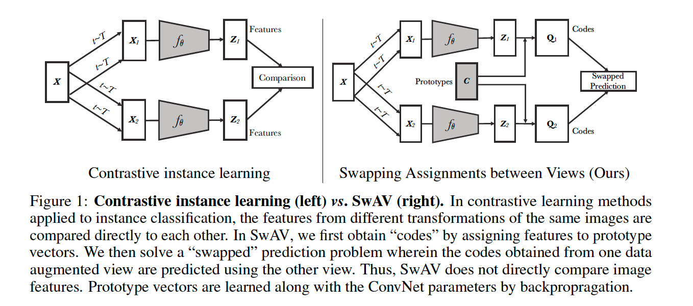
Enforce consistency between codes from different augmentations of the same image

( caution : do not consider the codes as a target, but only enforce consistent mapping )

Compute a code from an augmented version of image

& predict this code from augmented versions of the same image

Step 1) 2 image features input : \(\mathbf{z}_{t}\) and \(\mathbf{z}_{s}\)

• from different augmentation ( but same image )

Step 2) compute their codes : \(\mathbf{q}_{t}\) and \(\mathbf{q}_{s}\)

• by matching these features to a set of \(K\) prototypes \(\left\{\mathbf{c}_{1}, \ldots, \mathbf{c}_{K}\right\}\).

Step 3) “swapped” prediction problem

• \(L\left(\mathbf{z}_{t}, \mathbf{z}_{s}\right)=\ell\left(\mathbf{z}_{t}, \mathbf{q}_{s}\right)+\ell\left(\mathbf{z}_{s}, \mathbf{q}_{t}\right)\).
  • \(\ell(\mathbf{z}, \mathbf{q})\) : fit between features \(\mathbf{z}\) and a code \(\mathbf{q}\)

(1) Online Clustering

(1) image : \(\mathbf{x}_{n}\)

(2) augmented image : \(\mathbf{x}_{n t}\)…. applying a transformation \(t\)

(3) mapped to a vector representation : \(\mathbf{z}_{n t}=f_{\theta}\left(\mathbf{x}_{n t}\right) / \mid \mid f_{\theta}\left(\mathbf{x}_{n t}\right) \mid \mid _{2}\)

(4) compute code : \(\mathbf{q}_{n t}\)

• by mapping \(\mathbf{z}_{n t}\) to a set of \(K\) trainable prototype vectors, \(\left\{\mathbf{c}_{1}, \ldots, \mathbf{c}_{K}\right\}\)
• \(\mathbf{C}\) : matrix whose columns are the \(\mathbf{c}_{1}, \ldots, \mathbf{c}_{k}\)

\(\rightarrow\) how to compute these \(\mathbf{q}_{n t}\) & update \(\left\{\mathbf{c}_{1}, \ldots, \mathbf{c}_{K}\right\}\) ??

Swapped Prediction problem

Loss Function

• \(L\left(\mathbf{z}_{t}, \mathbf{z}_{s}\right)=\ell\left(\mathbf{z}_{t}, \mathbf{q}_{s}\right)+\ell\left(\mathbf{z}_{s}, \mathbf{q}_{t}\right)\).

  • \(\ell\left(\mathbf{z}_{t}, \mathbf{q}_{s}\right)\) : predicting the code \(\mathbf{q}_{s}\) from the feature \(\mathbf{z}_{t}\)
  • \(\ell\left(\mathbf{z}_{s}, \mathbf{q}_{t}\right)\) : predicting the code \(\mathbf{q}_{t}\) from the feature \(\mathbf{z}_{s}\)

  ( each term : CE loss )

  • \(\ell\left(\mathbf{z}_{t}, \mathbf{q}_{s}\right)=-\sum_{k} \mathbf{q}_{s}^{(k)} \log \mathbf{p}_{t}^{(k)}, \quad \text { where } \quad \mathbf{p}_{t}^{(k)}=\frac{\exp \left(\frac{1}{\tau} \mathbf{z}_{t}^{\top} \mathbf{c}_{k}\right)}{\sum_{k^{\prime}} \exp \left(\frac{1}{\tau} \mathbf{z}_{t}^{\top} \mathbf{c}_{k^{\prime}}\right)}\).

Total Loss for “Swapped Prediction problem”

( over all the images and pairs of data augmentations )

• \(-\frac{1}{N} \sum_{n=1}^{N} \sum_{s, t \sim \mathcal{T}}\left[\frac{1}{\tau} \mathbf{z}_{n t}^{\top} \mathbf{C} \mathbf{q}_{n s}+\frac{1}{\tau} \mathbf{z}_{n s}^{\top} \mathbf{C} \mathbf{q}_{n t}-\log \sum_{k=1}^{K} \exp \left(\frac{\mathbf{z}_{n t}^{\top} \mathbf{c}_{k}}{\tau}\right)-\log \sum_{k=1}^{K} \exp \left(\frac{\mathbf{z}_{n s}^{\top} \mathbf{c}_{k}}{\tau}\right)\right]\).

\(\rightarrow\) optimize w.r.t \(\theta\) & \(\mathbf{C}\)

Computing Codes Online

\(\rightarrow\) compute the codes using only the image features within a batch , using prototypes \(\mathbf{C}\)

( common prototypes \(\mathbf{C}\) are used across different batch )

Induce that all the examples in a batch are equally partitioned by the prototypes

\(\rightarrow\) preventing the trivial solution where every image has the same code

Notation

«««< HEAD:_posts/2022-05-20-(CL_paper9)SwAV.md

• Feature vectors : \(\mathbf{Z}=\left[\mathbf{z}_{1}, \ldots, \mathbf{z}_{B}\right]\)
• Codes : \(\mathbf{Q}=\left[\mathbf{q}_{1}, \ldots, \mathbf{q}_{B}\right]\)

• Prototype vectors : \(\mathbf{C}=\left[\mathbf{c}_{1}, \ldots, \mathbf{c}_{K}\right]\)

• feature vectors : \(\mathbf{Z}=\left[\mathbf{z}_{1}, \ldots, \mathbf{z}_{B}\right]\)
• prototypes : \(\mathbf{C}=\left[\mathbf{c}_{1}, \ldots, \mathbf{c}_{K}\right]\)
• codes : \(\mathbf{Q}=\left[\mathbf{q}_{1}, \ldots, \mathbf{q}_{B}\right]\)

  9b5515f0 (swav):_posts/2022-05-20-(CL_paper8)SwAV.md

\(\rightarrow\) optimize \(\mathbf{Q}\) to maximize similarity between features & prototypes

( = \(\max _{\mathbf{Q} \in \mathcal{Q}} \operatorname{Tr}\left(\mathbf{Q}^{\top} \mathbf{C}^{\top} \mathbf{Z}\right)+\varepsilon H(\mathbf{Q})\) )

Loss Function for “Computing Codes Online”

\(\max _{\mathbf{Q} \in \mathcal{Q}} \operatorname{Tr}\left(\mathbf{Q}^{\top} \mathbf{C}^{\top} \mathbf{Z}\right)+\varepsilon H(\mathbf{Q})\).

• \(H\) : entropy function
  • \(H(\mathbf{Q})=-\sum_{i j} \mathbf{Q}_{i j} \log \mathbf{Q}_{i j}\).
• \(\varepsilon\) : parameter that controls the smoothness of the mapping
  • high \(\varepsilon\) : rivial solution where all samples collapse into an unique representation
  • thus, keep it low

[ Enforcing Equal Partition ] ( Asano et al. [2] )

• by constraining the matrix \(Q\) to belong to the transportation polytope

• (this paper) restrict the transportation polytope to the minibatch :

  • \(\mathcal{Q}=\left\{\mathbf{Q} \in \mathbb{R}_{+}^{K \times B} \mid \mathbf{Q} \mathbf{1}_{B}=\frac{1}{K} \mathbf{1}_{K}, \mathbf{Q}^{\top} \mathbf{1}_{K}=\frac{1}{B} \mathbf{1}_{B}\right\}\).

  \(\rightarrow\) enforce that on average each prototype is selected at least \(\frac{B}{K}\) times in the batch.

• solution : continuous solution \(\mathbf{Q}^{*}\) is obtained

  \(\rightarrow\) round up to get discrete code

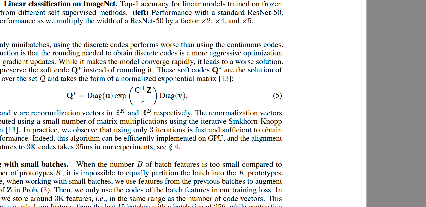
Details :

• ( in online setting ) discrete codes performs worse than using the continuous codes.

  ( \(\because\) rounding is a more aggressive optimization step than gradient updates )

  \(\rightarrow\) makes the model converge rapidly, but leads to a worse solution.

• thus, use the SOFT code \(\mathbf{Q}^{*}\)

  • \(\mathbf{Q}^{*}=\operatorname{Diag}(\mathbf{u}) \exp \left(\frac{\mathbf{C}^{\top} \mathbf{Z}}{\varepsilon}\right) \operatorname{Diag}(\mathbf{v})\).
    • where \(\mathbf{u}\) and \(\mathbf{v}\) are renormalization vectors in \(\mathbb{R}^{K}\) and \(\mathbb{R}^{B}\) respectively.

Working with small batches

• when \(B\) ( number of batch features ) < \(K\)

  \(\rightarrow\) impossible to equally partition the batch into \(K\) prototype

• solution : use features from the previous batches to augment the size of \(\mathbf{Z}\)

  ( but for loss…. only codes in the batch )

  • store around \(3 \mathrm{~K}\) features

(2) Multi-crop

( = Augmenting views with smaller images )

Problem of random crops :

• increasing the number of crops or “views” quadratically increases the memory and compute requirements

Solution : use two standard resolution crops

• sample \(V\) additional low resolution crops

  \(\rightarrow\) ensures only a small increase in the compute cost

BEFORE vs AFTER

• [BEFORE] \(L\left(\mathbf{z}_{t}, \mathbf{z}_{s}\right)=\ell\left(\mathbf{z}_{t}, \mathbf{q}_{s}\right)+\ell\left(\mathbf{z}_{s}, \mathbf{q}_{t}\right)\).
• [AFTER] \(L\left(\mathbf{z}_{t_{1}}, \mathbf{z}_{t_{2}}, \ldots, \mathbf{z}_{t_{V+2}}\right)=\sum_{i \in\{1,2\}} \sum_{v=1}^{V+2} \mathbf{1}_{v \neq i} \ell\left(\mathbf{z}_{t_{v}}, \mathbf{q}_{t_{i}}\right) .\).

4. Main Results

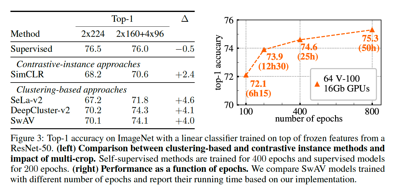
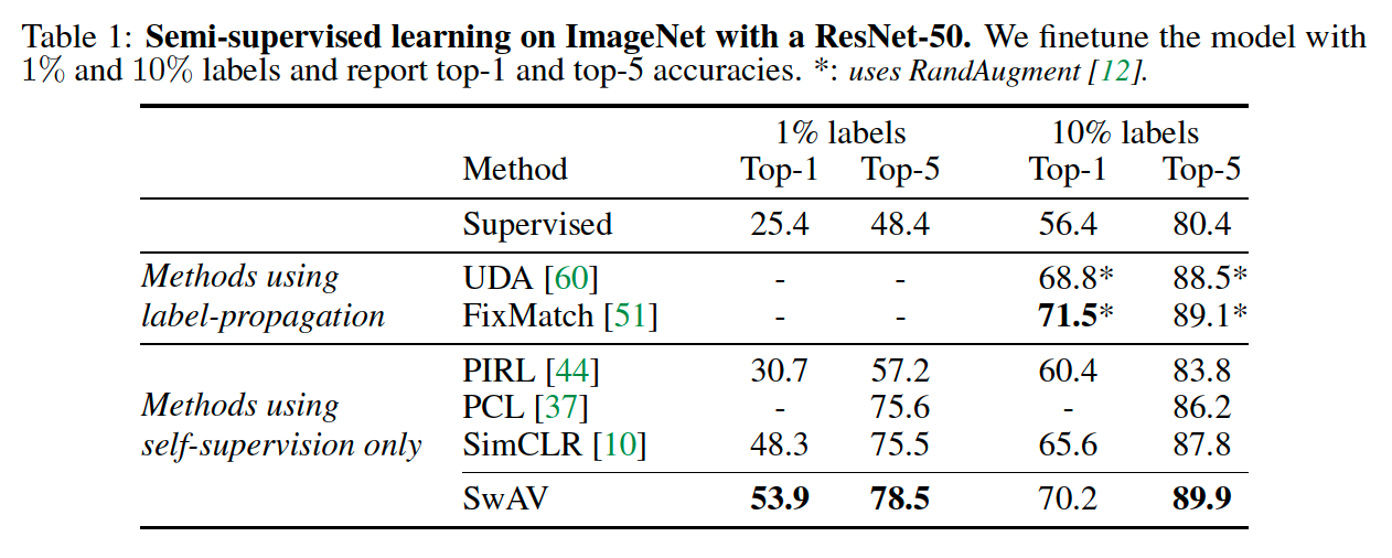
(1) Evaluating the unsupervised features on ImageNet

Settings : features of ResNet-50

2 experiments

• (1) linear classification on frozen features
• (2) semi-supervised learning by finetuning with few labels

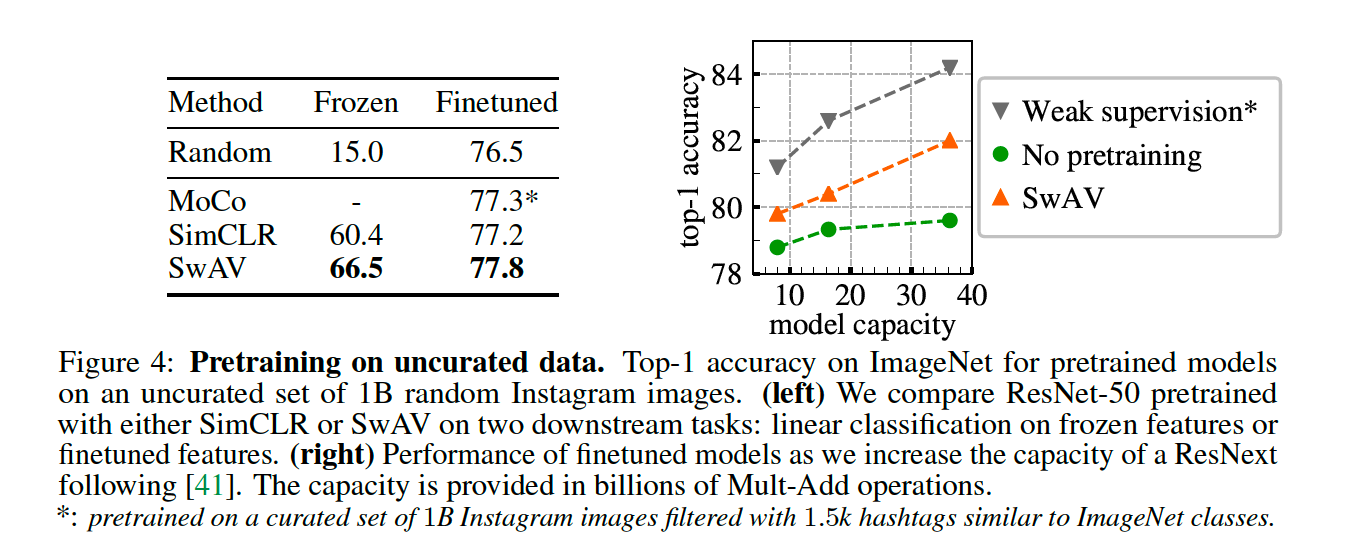
(2) Transferring unsupervised features to downstream tasks

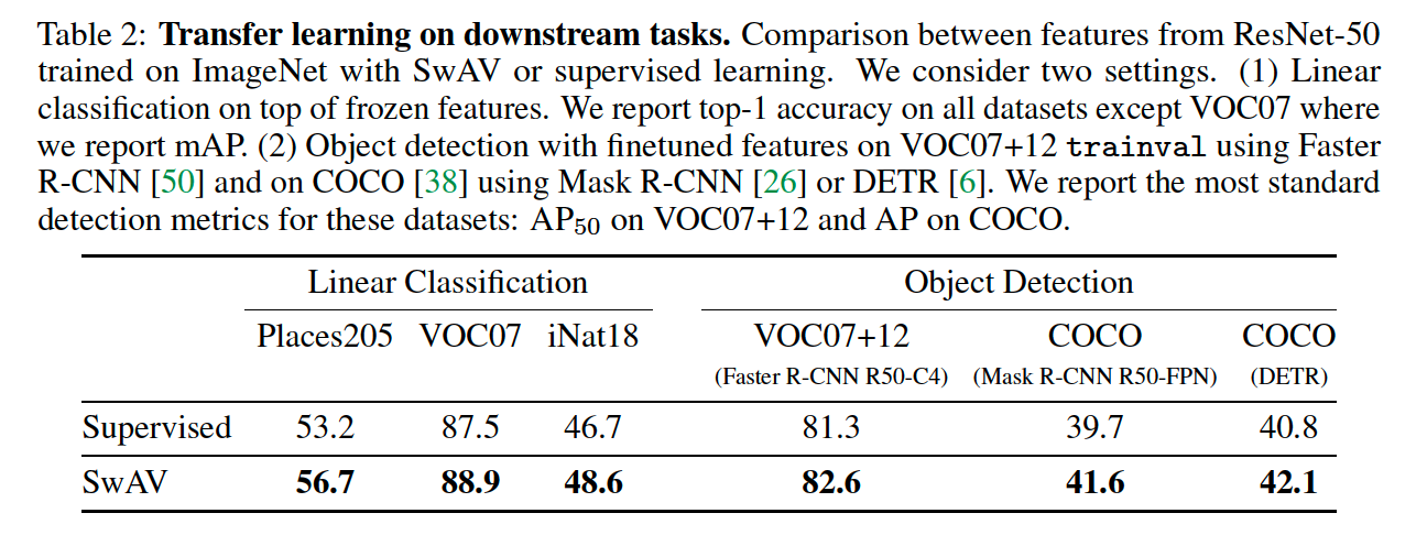
• outperforms supervised features on all three datasets

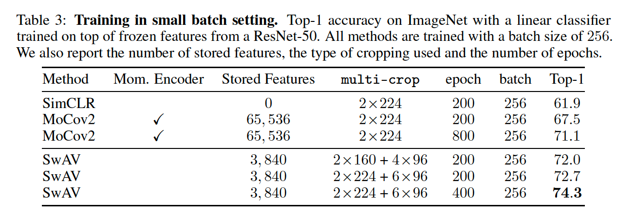
(3) Training with small batches

SwAV maintains SOTA performance even when trained in the small batch setting

5. Ablation Study