(paper 38) i-Mix

$i$-Mix: A Domain-Agnostic Strategy for Contrastive Representation Learning

Contents

1. Abstract
2. Introduction
3. Approach
   1. MixUp
   2. \(i\)-Mix
4. Application
   1. SimCLR
   2. MoCo
   3. BYOL

0. Abstract

i-Mix

• simple & effective domain agnostic regularization strategy
• to improve contrastive RL

• cast contrastive RL as training a non-parametric calssifier, by assigning a unique virtual class to each data in a batch

• data instances are mixed in both INPUT & VIRTUAL LABEL spaces

short summary = MixUp + Contrastive Learning

1. Introduction

propose instance Mix (i-Mix)

• domain agnostic regularization strategy
• introduce virtual labels in a batch
  • mix data instances & their corresponding virtual labels

apply them to SimCLR, MoCo, BYOL

2. Approach

• review MixUp ( in supervised learning )

• present i-Mix ( in contrastive learning )

Notation

• \(\mathcal{X}\) : data space
• \(\mathbb{R}^D\) : \(D\)-dim embedding space
• model \(f: \mathcal{X} \rightarrow \mathbb{R}^D\)
  • \(f_i=f\left(x_i\right)\) and \(\tilde{f}_i=f\left(\tilde{x}_i\right)\)

(1) MixUp ( in supervised learning )

Notation

• \(y_i \in\{0,1\}^C\) : one-hot label for \(x_i\)

  • \(C\) : # of classes

• linear classifier :

  • consists of weight vectors \(\left\{w_1, \ldots, w_C\right\}\), where \(w_c \in \mathbb{R}^D .\)

• Cross-entropy loss :

  • \(\ell_{\text {Sup }}\left(x_i, y_i\right)=-\sum_{c=1}^C y_{i, c} \log \frac{\exp \left(w_c^{\top} f_i\right)}{\sum_{k=1}^C \exp \left(w_k^{\top} f_i\right)}\).

  • problem of CE loss : overconfident

    • solutions : label smoothing, adversarial traning, confidence calibration …

Mixup

• effective regularization, without much computational overhead
• conducts a linear interpolation of 2 instances, both in \(x\) & \(y\)
• notation :
  • \(\ell_{\mathrm{Sup}}^{\mathrm{MixUp}}\left(\left(x_i, y_i\right),\left(x_j, y_j\right) ; \lambda\right)=\ell_{\text {Sup }}\left(\lambda x_i+(1-\lambda) x_j, \lambda y_i+(1-\lambda) y_j\right)\).
    • \(\lambda \sim \operatorname{Beta}(\alpha, \alpha)\) : mixing coefficient

(2) \(i\)-Mix ( in contrastive learning )

\(i\)-Mix = instance mix

• instead of mixing class labels, interpolates their virtual labels

Notation

• \(\mathcal{B}=\left\{\left(x_i, \tilde{x}_i\right)\right\}_{i=1}^N\) : batch of data pairs
  • \(N\) : batch size
  • \(x_i, \tilde{x}_i \in \mathcal{X}\) : 2 views of same data
• pos & neg : \(\tilde{x}_i\) and \(\tilde{x}_{j \neq i}\)
• model \(f\) : embedding function
  • output of \(f\) is \(\mathrm{L} 2\)-normalized
• \(v_i \in\{0,1\}^N\) : virtual label of \(x_i\) & \(\tilde{x_i}\) in batch \(\mathcal{B}\)
• where \(v_{i, i}=1\) and \(v_{i, j \neq i}=0\)

General sample-wise contrastive loss with virtual labels : \(\ell\left(x_i, v_i\right)\)

• \(\ell^{i-\operatorname{Mix}}\left(\left(x_i, v_i\right),\left(x_j, v_j\right) ; \mathcal{B}, \lambda\right)=\ell\left(\operatorname{Mix}\left(x_i, x_j ; \lambda\right), \lambda v_i+(1-\lambda) v_j ; \mathcal{B}\right)\).
  • (before) \(\lambda x_i+(1-\lambda) x_j\) \(\rightarrow\) (after) \(\operatorname{Mix}\left(x_i, x_j ; \lambda\right)\)
  • (before) \(\lambda y_i+(1-\lambda) y_j\) \(\rightarrow\) (after) \(\lambda v_i+(1-\lambda) v_j\)

\(\operatorname{Mix}\left(x_i, x_j ; \lambda\right)\) : general version

Example )

• \(\operatorname{MixUp}\left(x_i, x_j ; \lambda\right)=\lambda x_i+(1-\lambda) x_j\) .

• \(\operatorname{CutMix}\left(x_i, x_j ; \lambda\right)=M_\lambda \odot x_i+\left(1-M_\lambda\right) \odot x_j\).

  • used when data values have a spatial correlation with neighbors
  • \(M_\lambda\) : binary mask filtering out region ( whose relative area is \((1-\lambda)\) )

  \(\rightarrow\) not valid when no spatial correlation

\(\rightarrow\) use MiXUP for \(i\)-Mix formulations

3. Application

(1) SimCLR

loss function

• \(\ell_{\operatorname{SimCLR}}\left(x_i ; \mathcal{B}\right)=-\log \frac{\exp \left(s\left(f_i, f_{(N+i) \bmod 2 N}\right) / \tau\right)}{\sum_{k=1, k \neq i}^{2 N} \exp \left(s\left(f_i, f_k\right) / \tau\right)}\).

i-Mix is not directly applicable

( \(\because\) virtual labels are defined differently for each anchor )

\(\rightarrow\) solution : simplify the formulation of SimCLR, by excluding anchors from negative samples

(with virtual labels) N-way discrimination loss

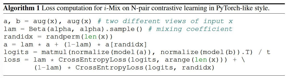
• \(\ell_{\mathrm{N}-\mathrm{pair}}\left(x_i, v_i ; \mathcal{B}\right)=-\sum_{n=1}^N v_{i, n} \log \frac{\exp \left(s\left(f_i, \tilde{f}_n\right) / \tau\right)}{\sum_{k=1}^N \exp \left(s\left(f_i, \tilde{f}_k\right) / \tau\right)}\).
  • whole batch is used to calculate loss for each instance!

Loss function ( for pairs \(\mathcal{B}=\left\{\left(x_i, \tilde{x}_i\right)\right\}_{i=1}^N\) ) ( with \(i\)-Mix )

• \(\ell_{\mathrm{N} \text {-pair }}^{i \text {-Mix }}\left(\left(x_i, v_i\right),\left(x_j, v_j\right) ; \mathcal{B}, \lambda\right)=\ell_{\mathrm{N} \text {-pair }}\left(\lambda x_i+(1-\lambda) x_j, \lambda v_i+(1-\lambda) v_j ; \mathcal{B}\right)\).

(2) MoCo

( Limitations of SimCLR )

# of negative samples affect the quality

\(\rightarrow\) \(\therefore\) SimCLR : requires large batch size

MoCo

• use memory bank \(\mathcal{M}=\left\{\mu_k\right\}_{k=1}^K\)
  • queue of previously extracted embeddings
  • updated in FIFO way
• EMA model
  • parameters are updated as \(\theta_{f_{\mathrm{EMM}}} \leftarrow m \theta_{f_{\mathrm{EMA}}}+(1-m) \theta_f\)

Loss function :

• \(\ell_{\mathrm{MoCo}}\left(x_i ; \mathcal{B}, \mathcal{M}\right)=-\log \frac{\exp \left(s\left(f_i, \tilde{f}_i^{\mathrm{EMA}}\right) / \tau\right)}{\exp \left(s\left(f_i, \tilde{f}_i^{\mathrm{EMA}}\right) / \tau\right)+\sum_{k=1}^K \exp \left(s\left(f_i, \mu_k\right) / \tau\right)}\).

i-Mix is not directly applicable

( \(\because\) virtual labels are defined differently for each anchor )

\(\rightarrow\) solution : simplify the formulation of SimCLR, by excluding anchors from negative samples

virtual label for MoCo : \(\tilde{v}_i \in\{0,1\}^{N+K}\)

(with virtual labels) (N+K)-way discrimination loss

• \(\ell_{\mathrm{MoCo}}\left(x_i, \tilde{v}_i ; \mathcal{B}, \mathcal{M}\right)=-\sum_{n=1}^N \tilde{v}_{i, n} \log \frac{\exp \left(s\left(f_i, \tilde{f}_n^{\mathrm{EMA}}\right) / \tau\right)}{\sum_{k=1}^N \exp \left(s\left(f_i, \tilde{f}_k^{\mathrm{EMA}}\right) / \tau\right)+\sum_{k=1}^K \exp \left(s\left(f_i, \mu_k\right) / \tau\right)}\).

Loss function ( for pairs \(\mathcal{B}=\left\{\left(x_i, \tilde{x}_i\right)\right\}_{i=1}^N\) ) ( with \(i\)-Mix )

• \(\ell_{\mathrm{MoCo}}^{i-\mathrm{Mix}}\left(\left(x_i, \tilde{v}_i\right),\left(x_j, \tilde{v}_j\right) ; \mathcal{B}, \mathcal{M}, \lambda\right)=\ell_{\mathrm{MoCo}}\left(\lambda x_i+(1-\lambda) x_j, \lambda \tilde{v}_i+(1-\lambda) \tilde{v}_j ; \mathcal{B}, \mathcal{M}\right)\).

(3) BYOL

descriptions of BYOL

• without contrasting negative pairs

• predict a view embedded with EMA model \(\tilde{f}_i^{\mathrm{EMA}}\) from its embedding \(f_i\)
• prediction layer \(g\)
  • difference between \(g\left(f_i\right)\) and \(\tilde{f}_i^{\mathrm{EMA}}\) is learned to be minimized

loss function :

• \(\ell_{\text {BYOL }}\left(x_i, \tilde{x}_i\right)= \mid \mid g\left(f_i\right) / \mid \mid g\left(f_i\right) \mid \mid -\tilde{f}_i / \mid \mid \tilde{f}_i \mid \mid \mid \mid ^2=2-2 \cdot s\left(g\left(f_i\right), \tilde{f}_i\right)\).

to derive \(i\)-Mix in BYOL…

• let \(\tilde{F}=\left[\tilde{f}_1 / \mid \mid \tilde{f}_1 \mid \mid , \ldots, \tilde{f}_N / \mid \mid \tilde{f}_N \mid \mid \right] \in \mathbb{R}^{D \times N}\)

  ( collection of L2-normalized embedding vectors of 2nd views )

  • \(\tilde{f}_i / \mid \mid \tilde{f}_i \mid \mid =\tilde{F} v_i\).

(with virtual labels) loss function

• \(\ell_{\mathrm{BYOL}}\left(x_i, v_i ; \mathcal{B}\right)= \mid \mid g\left(f_i\right) / \mid \mid g\left(f_i\right) \mid \mid -\tilde{F} v_i \mid \mid ^2=2-2 \cdot s\left(g\left(f_i\right), \tilde{F} v_i\right)\).

Loss function ( for pairs \(\mathcal{B}=\left\{\left(x_i, \tilde{x}_i\right)\right\}_{i=1}^N\) ) ( with \(i\)-Mix )

• \(\ell_{\mathrm{BYOL}}^{i \text {-Mix }}\left(\left(x_i, v_i\right),\left(x_j, v_j\right) ; \mathcal{B}, \lambda\right)=\ell_{\mathrm{BYOL}}\left(\lambda x_i+(1-\lambda) x_j, \lambda v_i+(1-\lambda) v_j ; \mathcal{B}\right)\).