
( 참고 : 패스트 캠퍼스 , 한번에 끝내는 컴퓨터비전 초격차 패키지 )
Object Detection - RCNN
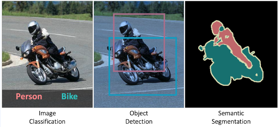
1. Visual Recognition Tasks
- Image Classification
- Object Detection : “bounding box”
- Semantic Segmentation : “pixel-level”
2. Naive Approach
Object Detection (OD) = (1) + (2)
- (1) Box Localization ( via object proposals )
- ex 1) Selective Search for Object Detection ( IJCV 2013 )
- ex 2) Edge Boxes : Locating Object Proposals from Edges ( ECCV 2014 )
- (2) Box Classification ( via CNN )
3. RCNN (2014)
( Girshick et al., Rich Feature Hierarchies for Accurate Object Detection and Semantic Segmentation, CVPR 2014 )
RCNN = Region-based CNN
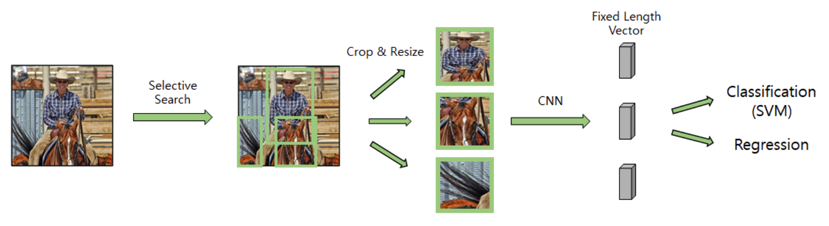
(1) Summary
-
2 stage detector
-
stage # 1 : region proposal
-
stage # 2 : classification
-
-
a) Region proposal :
-
2,000 proposed regions per image
-
crop 2,000 regions into same size
( for a fixed-length vector, for regression & classification )
-
put 2,000 regions to CNN ( \(\rightarrow\) very slow )
-
-
b) Regression & Classification :
- with 2,000 fixed-length vectors, do regression & classification
- Classification
- binary SVM x (num_classes+1) … for background
- Regression
- IoU >= 0.3 : positive
- IoU < 0.3 : negative
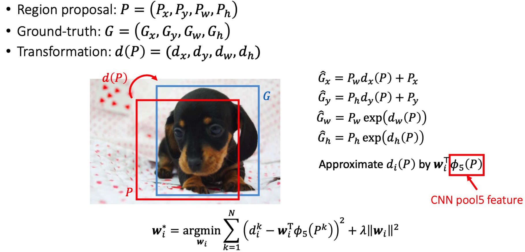
(2) Regression
Regression = Learning a transformation of bounding box
(3) Loss Function
\(\begin{aligned} t_{x} &=\left(g_{x}-p_{x}\right) / p_{w} \\ t_{y} &=\left(g_{y}-p_{y}\right) / p_{h} \\ t_{w} &=\log \left(g_{w} / p_{w}\right) \\ t_{h} &=\log \left(g_{h} / p_{h}\right) \end{aligned}\).
\(\mathcal{L}_{\mathrm{reg}}=\sum_{i \in\{x, y, w, h\}}\left(t_{i}-d_{i}(\mathbf{p})\right)^{2}+\lambda \mid \mid \mathbf{w} \mid \mid ^{2}\).
4. Fast RCNN
( Girshick, Ross. “Fast R-CNN: Fast Region-based Convolutional Networks for object detection.” Internation Conference on Computer Vision,(ICCV). 2015. )
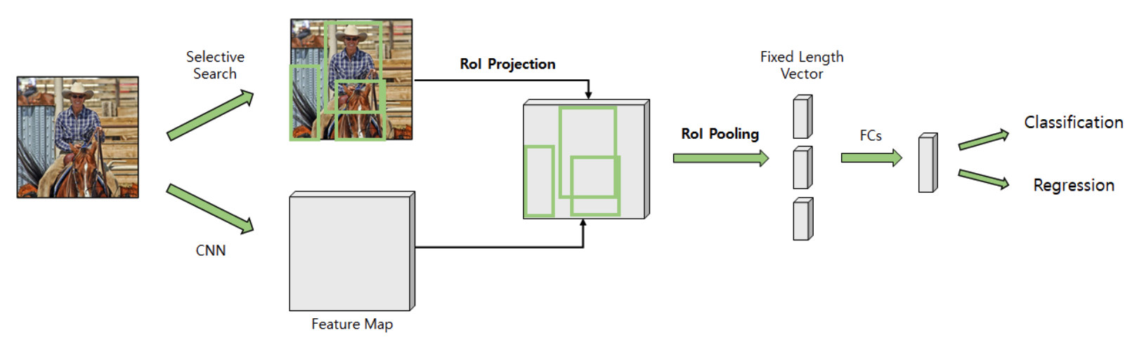
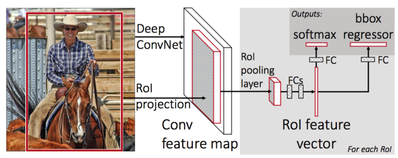
Solve the problem of slow speed of RCNN
RCNN vs Fast RCNN
-
common ) Region proposal using selective search
-
difference # 1 ) SPEED
-
RCNN :
- step 1) 2,000 region proposals
- step 2) crop 2,000 region proposals
- step 3) CNN 2,000 times ( with proposed regions )
-
Fast-RCNN
-
step 1-1) 2,000 region proposals
step 1-2) CNN 1 time ( with original image )
-
step 2) crop regions from feature map ( RoI projection )
-
-
-
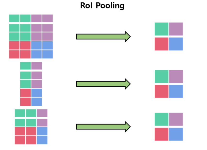
difference # 2 ) RoI Pooling
-
Why RoI Pooling??
-
no need for fixed length vector for CNN Input!
( just need fixed length for FC input )
-
Thus, RoI Pooling after RoI Projection!
-
-
-
difference # 3 ) Classification
- instead of SVM, use FC layer
(1) Roi Pooling
(2) Loss Function
\(\begin{aligned} \mathcal{L}\left(p, u, t^{u}, v\right) &=\mathcal{L}_{\mathrm{cls}}(p, u)+\mathbb{1}[u \geq 1] \mathcal{L}_{\mathrm{box}}\left(t^{u}, v\right) \\ \mathcal{L}_{\mathrm{cls}}(p, u) &=-\log p_{u} \\ \mathcal{L}_{\mathrm{box}}\left(t^{u}, v\right) &=\sum_{i \in\{x, y, w, h\}} L_{1}^{\text {smooth }}\left(t_{i}^{u}-v_{i}\right) \end{aligned}\).
- where \(L_{1}^{\mathrm{smooth}}(x)= \begin{cases}0.5 x^{2} & \text { if } \mid x \mid <1 \\ \mid x \mid -0.5 & \text { otherwise }\end{cases}\).
5. Faster RCNN
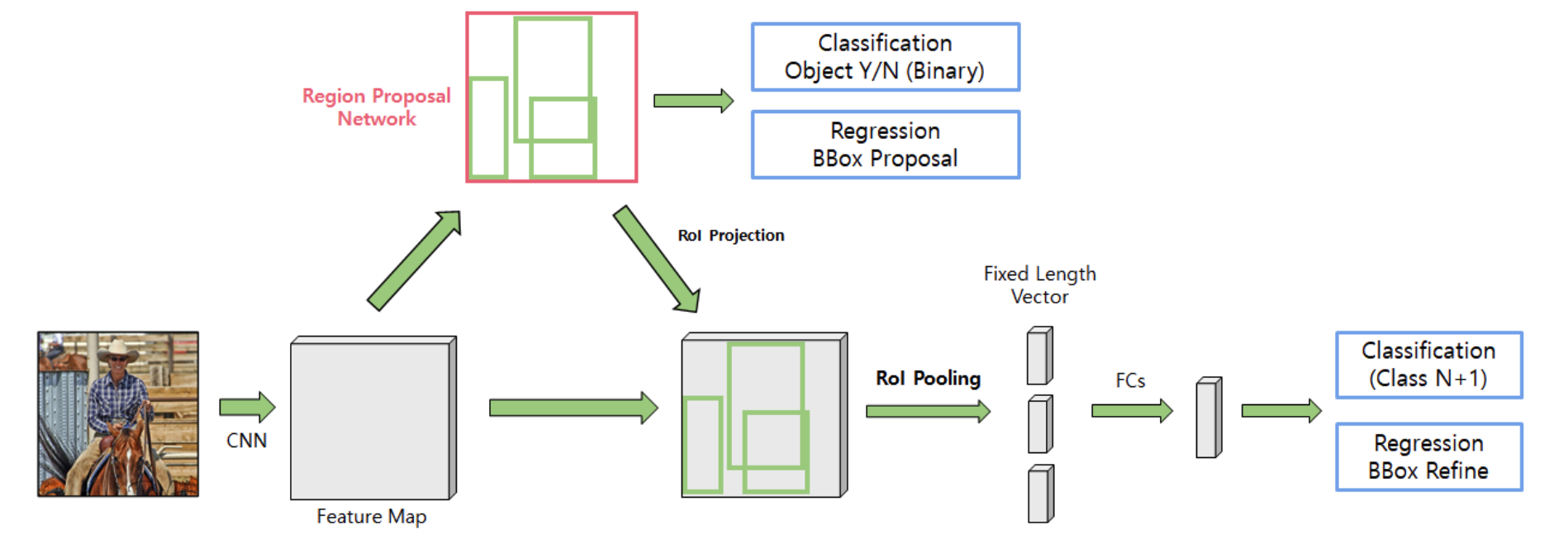
Solve the problem of selective search of RCNN/Fast RCNN
- selective search : on CPU -> bottleneck!
Faster RCNN : end-to-end
-
region proposal inside CNN, using GPU
-
Process
-
step 1) CNN with original image
-
step 2) input feature map to RPN (Region Proposal Network)
( use these output region proposals, instead of selective search )
-
below are same
-
Two Additional Loss ( of RPN )
- (Loss 1) Classification Loss
- (Loss 2) Box regression Loss
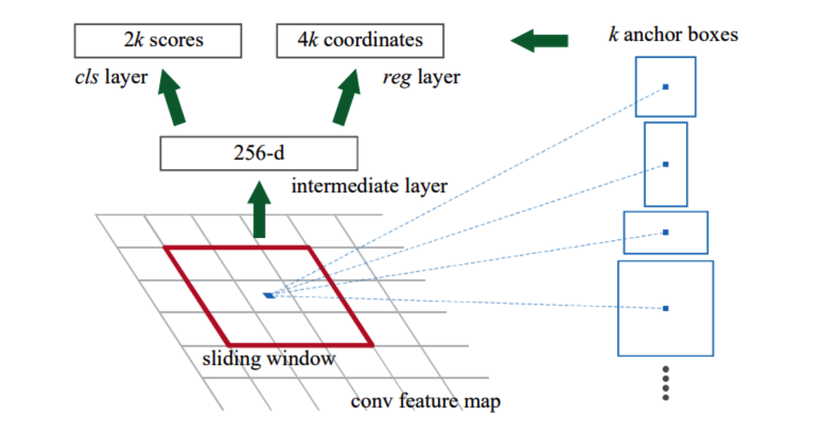
(1) RPN (Region Proposal Network)
-
Input : 7x7xC Feature Map
-
Kernel Size : 3 x 3 filter
-
Number of anchor boxes : K (=9)
- Output : 7x7x6K Feature Map
- 6k = 2k + 4k
- 2K : whether object is foreground/background
- 4K : (X,Y,W,H)
- 6k = 2k + 4k
- $p^{*}=f(x)=\left{\begin{aligned}
-1, & \text { if IoU }<0.3
1, & \text { if IoU }>0.7
0, & \text { otherwise } \end{aligned}\right.$.
(2) Loss Function
\(\begin{aligned} \mathcal{L} &=\mathcal{L}_{\mathrm{cls}}+\mathcal{L}_{\mathrm{box}} \\ \mathcal{L}\left(\left\{p_{i}\right\},\left\{t_{i}\right\}\right) &=\frac{1}{N_{\mathrm{cls}}} \sum_{i} \mathcal{L}_{\mathrm{cls}}\left(p_{i}, p_{i}^{*}\right)+\frac{\lambda}{N_{\mathrm{box}}} \sum_{i} p_{i}^{*} \cdot L_{1}^{\text {smooth }}\left(t_{i}-t_{i}^{*}\right) \end{aligned}\).
- where \(\mathcal{L}_{\mathrm{cls}}\left(p_{i}, p_{i}^{*}\right)=-p_{i}^{*} \log p_{i}-\left(1-p_{i}^{*}\right) \log \left(1-p_{i}\right)\).