(paper 68) Contrastive and Non-Contrastive Self-Supervised Learning Recover Global and Local Spectral Embedding Methods

Contrastive and Non-Contrastive Self-Supervised Learning Recover Global and Local Spectral Embedding Methods

Contents

1. Abstract
2. Introduction
3. Notations & Background on SSL
   1. Dataset, Embedding and Relation Matrix
   2. VICReg
   3. SimCLR
   4. BarlowTwins
   5. Linear Algebra Notations

0. Abstract

Limitations of SSL

• theoretical foundations are limited

• method-specific
• fail to provide principled design guidelines to practitioners

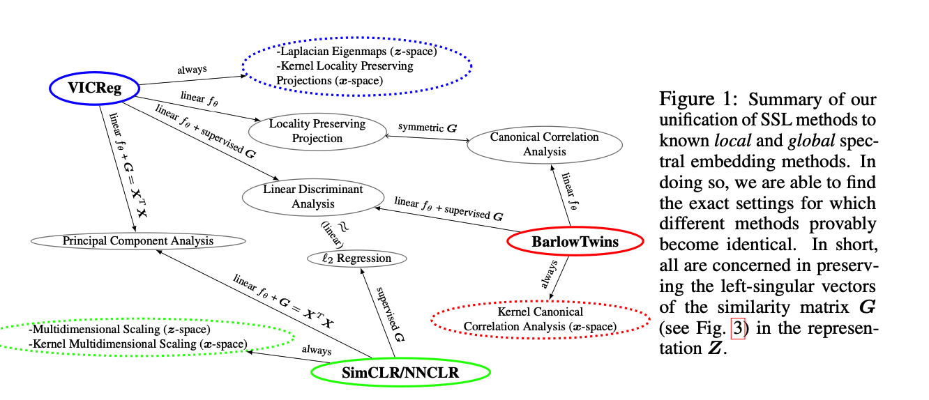
Propose a unifying framework,

under the helm of **spectral manifold learning **to address those limitations.

• Demonstrate that VICReg, SimCLR, BarlowTwins correspond to eponymous spectral methods such as Laplacian Eigenmaps, Multidimensional Scaling

• allow us to obtain (i), (ii), (iii) for each method

  • (i) the closed-form optimal representation
  • (ii) the closed-form optimal network parameters in the linear regime
  • (iii) the impact of the pairwise relations used during training on each of those quantities and on downstream task performances
  • (iv) the first theoretical bridge between contrastive and non-contrastive methods towards **global and local spectral embedding **methods respectively,

1. Introduction

Notation

• USL relies on \((\boldsymbol{X})\)
• SL relies on \((\boldsymbol{X}, \boldsymbol{Y})\)
• SSL relies on \((\boldsymbol{X}, \boldsymbol{G})\)
  • \(G\) : inter-sample relations
  • Matrix \(G\) is often constructed by DA of \(\boldsymbol{X}\)

\(\rightarrow\) Need for a principled theoretical understanding of SSL!

• to understand how well the learned transformation transfer to different downstream tasks

Understanding SSL theoretically : 3 appraoches

1. Studying the training dynamics and optimization landscapes in a linear network regime
   • e.g. validating some empirically found tricks as necessary conditions for stable gradient dynamics
2. Studying the role of individual SSL components separately
   • e.g. the projector and predictor networks
3. developing novel SSL criteria that often combine multiple interpretable objectives

Keypoint 1

all SSL methods’ optimal learn \(\boldsymbol{Z}\) ,

• whose top left singular vectors align with the ones of \(\boldsymbol{G}\),

• and that none of the SSL methods constrain the right-singular vectors of \(\boldsymbol{Z}\).

Keypoint 2

Guarantee that minimizing a SSL loss produces a representation that is optimal to solve a downstream task

Keypoint 3

Demonstrate that the

• [ VICReg ] \(\boldsymbol{Z}\) can be made full-rank while learning from \(\boldsymbol{G}\) by carefully selecting the loss hyperparameters
• [ SimCLR and BarlowTwins ] strictly enforce \(\operatorname{rank}(\boldsymbol{Z})=\operatorname{rank}(\boldsymbol{G})\), hinting at a possible advantage of VICReg when \(\boldsymbol{G}\) is misspecified

Keypoint 4

Connecting SSL methods to spectral embedding methods

\(\rightarrow\) improves our understanding and guide the design of novel SSL frameworks

\(\rightarrow\) demonstrate that contrastive and non-contrastive SSL corresponds to global and local spectral embedding methods respectively

Contributions

1. Closed-form optimal representation for SSL losses
2. Closed-form optimal network parameters for SSL losses with linear networks
3. Exact equivalence between SSL and spectral embedding methods
4. Optimality conditions of SSL representations on downstream tasks (Y )

2. Notations & Background on SSL

(1) Dataset, Embedding and Relation Matrix

Notation

• \(\boldsymbol{X} \triangleq\left[\boldsymbol{x}_1, \ldots, \boldsymbol{x}_N\right]^T \in \mathbb{R}^{N \times D}\) : Input samples
• \(\boldsymbol{G} \in\{0,1\}^{N \times N}\) : Known pairwise positive relation ( between those samples )
  • symmetric matrix, where \((\boldsymbol{G})_{i, j}=1\) iff samples \(\boldsymbol{x}_i\) and \(\boldsymbol{x}_j\) are known to be semantically related, and with 0 in the diagonal
  • positive samples = “views”
• \(\boldsymbol{Z} \in \mathbb{R}^{N \times K}\) : matrix of embeddings obtained from \(f_\theta\)-
  • \(\boldsymbol{Z} \triangleq\left[f_\theta\left(\boldsymbol{x}_1\right), \ldots, f_\theta\left(\boldsymbol{x}_N\right)\right]^T\).

Given a dataset \(\boldsymbol{X}^{\prime} \in \mathbb{R}^{N^{\prime} \times D^{\prime}}\) where commonly \(D=D^{\prime}\),

\(\rightarrow\) artificially constructs \(\boldsymbol{X}, \boldsymbol{G}\) from DA of \(\boldsymbol{X}^{\prime}\)

• \(\boldsymbol{X}=\left[\operatorname{View}_1\left(\boldsymbol{X}^{\prime}\right)^T, \ldots, \operatorname{View}_V\left(\boldsymbol{X}^{\prime}\right)^T\right]^T\).
  • row \(\left(\operatorname{View}_v\left(\boldsymbol{X}^{\prime}\right)\right)_{n, .}\) is viewed as similar to the same row of \(\left(\operatorname{View}_{v^{\prime}}\left(\boldsymbol{X}^{\prime}\right)\right)_{n, .}, \forall v \neq v^{\prime}\)
  • \(\mid V \mid\) \(= 2\) : only positive pairs are used
  • \(\operatorname{View}_c(),. c=1, \ldots, C\) operator is a sample-wise transformation

• entries of \(\boldsymbol{G}\) : positive for the samples that have been augmented form the same original sample

• shape of \(G\) : \(\left(V N^{\prime} \times V N^{\prime}\right)\)

N_original =  1000
V = 2

G = torch.zeros(N_original * V, N_original * V) 
i = torch.arange(0, N_original * V).repeat_interleave(V - 1) # row indices
j = (i + torch.arange(1, V).repeat(N_original * V) * N_original).remainder(N_original * V) # column indices
G[i,j] = 1 

print(G.shape)
print(i)
print(j)

torch.Size([2000, 2000])
tensor([   0,    1,    2,  ..., 1997, 1998, 1999])
tensor([1000, 1001, 1002,  ...,  997,  998,  999])

(2) VICReg

\(\mathcal{L}_{\text {vic }}=\alpha \sum_{k=1}^K \max \left(0,1-\sqrt{\operatorname{Cov}(\boldsymbol{Z})_{k, k}}\right)+\beta \sum_{j=1, j \neq k}^K \operatorname{Cov}(\boldsymbol{Z})_{k, j}^2+\frac{\gamma}{N} \sum_{i=1}^N \sum_{j=1}^N(\boldsymbol{G})_{i, j}\left\|\boldsymbol{Z}_{i, .}-\boldsymbol{Z}_{j, .}\right\|_2^2\).

computational complexity of \(\mathcal{O}\left(N K^2+P N K\right)\)

• \(P\) : average number of positive samples

  ( i.e. number of nonzeros elements in each row of \(\boldsymbol{G}\) )

• usually … \((P \ll K)\) \(\rightarrow\) the computational cost is dominated by the covariance matrix, \(\mathcal{O}\left(N K^2\right)\).

Settings :

N_original =  1000
V = 2
N = N_original*V
dim = 128

Z = torch.randn(N, dim)
C = torch.cov(Z.t()) 

Variance Loss : \(\sum_{k=1}^K \max \left(0,1-\sqrt{\operatorname{Cov}(\boldsymbol{Z})_{k, k}}\right)\)

var_loss = dim - torch.diag(C).clamp(1e-6, 1).sqrt().sum() 
print(torch.diag(C).shape)

torch.Size([128])

Covarinace Loss : \(\sum_{j=1, j \neq k}^K \operatorname{Cov}(\boldsymbol{Z})_{k, j}^2\)

cov_loss = 2 * torch.triu(C, diagonal=1).square().sum() 
print(torch.triu(C, diagonal=1).shape)

torch.Size([128, 128])

Invariance Loss : \(\frac{1}{N} \sum_{i=1}^N \sum_{j=1}^N(\boldsymbol{G})_{i, j}\left\|\boldsymbol{Z}_{i, .}-\boldsymbol{Z}_{j, .}\right\|_2^2\)

inv_loss =(Z[i]-Z[j]).square().sum(1).inner(G[i,j])/N 
print((Z[i]-Z[j]).shape)

torch.Size([2000, 128])

Overall loss :

loss = alpha * var_loss + beta * cov_loss + gamma * inv_loss 

(3) SimCLR

consists in two steps

• step 1) produces an estimate \(\widehat{\boldsymbol{G}}(\boldsymbol{Z})\) of the \(\boldsymbol{G}\) from \(\boldsymbol{Z}\)

  • \(\widehat{\boldsymbol{G}}(\boldsymbol{Z})\) : right-stochastic matrix ( \(\widehat{\boldsymbol{G}}(\boldsymbol{Z}) \mathbf{1}=\mathbf{1}\) )

  • ex) by using the cosine similarity

    \((\widehat{\boldsymbol{G}}(\boldsymbol{Z}))_{i, j}=\frac{e^{\operatorname{CoSim}\left(\boldsymbol{z}_i, \boldsymbol{z}_j\right) / \tau}}{\sum_{k=1, k \neq i}^N e^{\operatorname{CoSim}\left(\boldsymbol{z}_i, \boldsymbol{z}_k\right) / \tau}} \mathbf{1}_{\{i=j\}},\).

• step 2) encourages the elements of \(\widehat{G}(\boldsymbol{Z})\) and \(G\) to match

  • ex) InfoNCE loss

    \(\mathcal{L}_{\text {simCLR }}=\underbrace{-\sum_{i=1}^N \sum_{j=1}^N(\boldsymbol{G})_{i, j} \log (\widehat{\boldsymbol{G}}(\boldsymbol{Z}))_{i, j}}_{\text {cross-entropy between matrices }}\).

The only difference between SimCLR and its variants e.g. NNCLR

\(\rightarrow\) construction of \(\boldsymbol{G}\) when only given \(\boldsymbol{X}^{\prime}\)

computational complexity of \(\mathcal{O}\left(N^2\right)\)

• \(\because\) requires to compute all the pairwise similarities

Nevertheless, InfoNCE loss above can be easily computed as…

tau = 3
Z = torch.randn(N, dim)
I = torch.eye(N, N)

Z_renorm = torch.nn.functional.normalize(Z, dim=1)
cosim = Z_renorm @ Z_renorm.t() / tau 
off_diag = cosim[~I.bool()].reshape(N, N-1)

print(Z_renorm.shape)
print(cosim.shape)
print(off_diag.shape)

torch.Size([2000, 128])
torch.Size([2000, 2000])
torch.Size([2000, 1999])

loss = (G * (torch.logsumexp(off_diag, dim=1, keepdim=True) - cosim)).sum() 

print(G.shape)
print(torch.logsumexp(off_diag, dim=1, keepdim=True).shape)
print((G * (torch.logsumexp(off_diag, dim=1, keepdim=True) - cosim)).shape)
print(cosim.shape)

torch.Size([2000, 2000])
torch.Size([2000, 1])
torch.Size([2000, 2000])
torch.Size([2000, 2000])

(4) BarlowTwins

2 views of a dataset \(\boldsymbol{X}^{\prime}\) :

• data : \(\boldsymbol{X}_{\text {left }}\) & \(\boldsymbol{X}_{\text {right }}\)
• embeddings : \(\boldsymbol{Z}_{\text {left }}\) and \(\boldsymbol{Z}_{\text {right. }}\)
  • \(\boldsymbol{C}\) : \(K \times K\) cross-correlation matrix between \(\boldsymbol{Z}_{\text {left }}\) and \(\boldsymbol{Z}_{\text {right }}\)

The same row of those left/right matrices are the positive pairs

\(\mathcal{L}_{\mathrm{BT}}=\sum_{k=1}^K\left((\boldsymbol{C})_{k, k}-1\right)^2+\alpha \sum_{k^{\prime} \neq k}(\boldsymbol{C})_{k, k}^2, \alpha>0\).

• \((\boldsymbol{C})_{i, j}\) : measuring the cosmic btw the \(i^{\text {th }}\) column of \(\boldsymbol{Z}_{\text {left }}\) and the \(j^{\text {th }}\) column of \(\boldsymbol{Z}_{\text {right }}\)

• \((\boldsymbol{C})_{i, j}=\frac{\left\langle\left(\boldsymbol{Z}_{\text {left }}\right)_{., i},\left(\boldsymbol{Z}_{\text {right }}\right)_{., j}\right\rangle}{\left\|\left(\boldsymbol{Z}_{\text {left }}\right)_{., i}\right\|_2\left\|\left(\boldsymbol{Z}_{\text {right }}\right)_{., j}\right\|_2+\epsilon}\).

Computational complexity : \(\mathcal{O}\left(N K^2\right)\)

Z_left = torch.randn(N, dim)
Z_right = torch.randn(N, dim)
I = torch.eye(dim, dim)
eps = 1e-6
alpha = 0.1

Z_rrenorm = torch.nn.functional.normalize(Z_right, dim=0, eps=eps) 
Z_lrenorm = torch.nn.functional.normalize(Z_left, dim=0, eps=eps)

C = Z_lrenorm.t() @ Z_rrenorm 
print(C.shape)

loss = (C.diag() - 1).square().sum()+ alpha*C[~I.bool()].square().sum() 
print(loss)

torch.Size([128, 128])
tensor(129.5863)

Still possible to recover \(\boldsymbol{X}_{\text {left }}, \boldsymbol{X}_{\text {right }}\) for \(\mathcal{L}_{\mathrm{BT}}\) as below!

Ex) 5 data samples ( \(\boldsymbol{a}, \boldsymbol{b}, \boldsymbol{c}, \boldsymbol{d}, \boldsymbol{e}\) )

• \(\boldsymbol{a}, \boldsymbol{b}, \boldsymbol{c}\) are related to each other
• \(\boldsymbol{d}, \boldsymbol{e}\) are related to each other

2 data matrices :

• \(\boldsymbol{X}_{\text {left }}=[\boldsymbol{a}, \boldsymbol{a}, \boldsymbol{b}, \boldsymbol{b}, \boldsymbol{c}, \boldsymbol{c}, \boldsymbol{d}, \boldsymbol{e}]^T\).
• \(\boldsymbol{X}_{\mathrm{right}}=[\boldsymbol{b}, \boldsymbol{c}, \boldsymbol{a}, \boldsymbol{c}, \boldsymbol{a}, \boldsymbol{b}, \boldsymbol{e}, \boldsymbol{d}]^T\).

N_original =  1000
V = 2
N = N_original * V

X = torch.randn(N, dim)
G = torch.zeros(N, N) 
i = torch.arange(0, N).repeat_interleave(V - 1) 
j = (i + torch.arange(1, V).repeat(N) * N_original).remainder(N) 
G[i,j] = 1 

row_indices, col_indices = G.nonzero(as_tuple=True)
X_left = X[row_indices]  
X_right = X[col_indices] 
print(X_left.shape)
print(X_right.shape)

torch.Size([2000, 128])
torch.Size([2000, 128])

(5) Linear Algebra Notations

Singular Value Decomposition (SVD)

\(\boldsymbol{X}=\boldsymbol{U}_x \boldsymbol{\Sigma}_x \boldsymbol{V}_x^T\) :

• left singular vectors \(\boldsymbol{U}_x \in \mathbb{R}^{N \times N}\)
• singular values \(\boldsymbol{\Sigma}_x \in \mathbb{R}^{N \times D}\)
• right singular vectors \(\boldsymbol{V}_x \in \mathbb{R}^{D \times D}\) of \(\boldsymbol{X} \in \mathbb{R}^{N \times D}\)

\(\overline{\boldsymbol{U}}_x\) and \(\overline{\boldsymbol{V}}_x\) : left/right singular vectors, whose associated singular values are 0

\(\sigma_z\) : vector of singular values such as \(\boldsymbol{\Sigma}_z=\operatorname{diag}(\boldsymbol{\sigma})\)

Goal : Find the optimal \(\boldsymbol{Z}\) of \(\boldsymbol{X}\), whilst tying those methods to their spectral 드embedding counterpart.

Three findings :

1. Above methods recover exactly some flavors of famous spectral method
2. Spectral properties of optimal \(\boldsymbol{Z}\) of \(\boldsymbol{X}\) can be obtained in closed-form
3. Necessary & Sufficient conditions can be obtained to bounds the downstream task error fo those optimal \(\boldsymbol{Z}\)