
REST: Reciprocal Framework for Spatiotemporal-coupled Predictions
Contents
- Abstract
- Introduction
0. Abstract
proposes to jointly …
- (1) mine the “spatial” dependencies
- (2) model “temporal” patterns
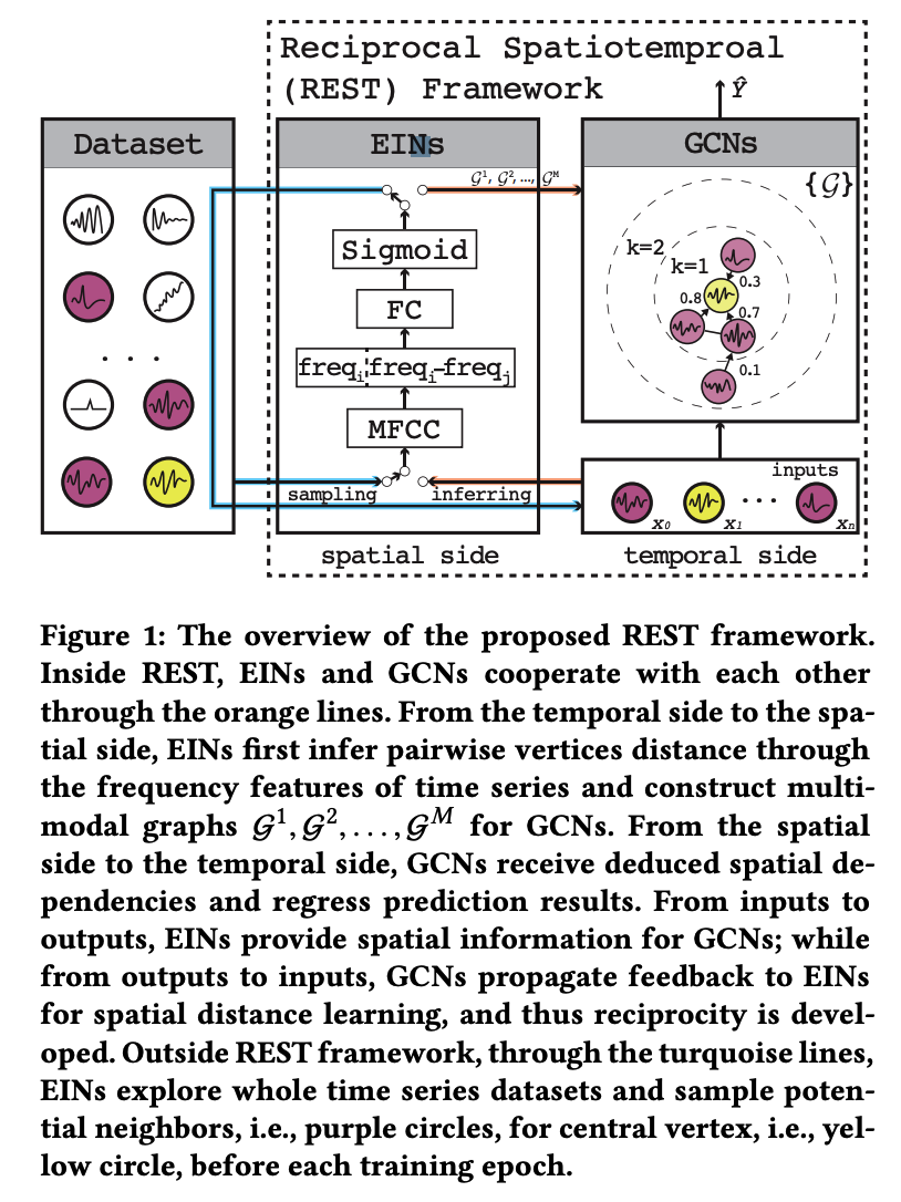
propose Reciprocal SpatioTemporal (REST)
-
introduces Edge Inference Networks (EINs) to couple with GCNs.
-
generate “multi-modal” directed weighted graphs to serve GCNs.
-
GCNs utilize these graphs ( = spatial dependencies ) to make predictions
& introduce feedback to optimize EINs
-
-
design a phased heuristic approach
- effectively stabilizes training procedure and prevents early-stop
1. Introduction
Problem : Domain knowledge is required to construct an accurate graph
\(\rightarrow\) not only COSTLY, but also SUB-OPTIMAL !
3 Challenges in “spatio temporal-coupled” predictions
-
(1) Data property aspect
-
1-1) lacks existing edge labels
-
1-2) the information of TS may be limited and noisy
\(\rightarrow\) making it difficult to find the distance among TS & cluster them as a graph
-
-
(2) Learning aspect
- without effective inductive bias, a model is easy to overfit the noises & the learning procedure may become unstable
-
(3) Practicality aspect
-
mining potential links between two arbitrary TS pairs also brings significant computational burden
( as the possible links are in \(n^2\) order )
-
Existing research
- (1) based on “predefined” graph structure
- (2) “infer potential links” with strong domain knowledge
propose a novel Reciprocal Spatiotemporal (REST) framework
\(\rightarrow\) to address 3 challenges
REST
consists of 2 integral parts
- (1) Edge Inference Networks (EINs)
- for mining “spatial” dependencies among TS
- (2) GCNs ( e.g., DCRNNs )
- for making “spatio temporal” prediction
Spatial \(\rightarrow\) Temporal
- Spatial dependencies inferred by EINs promote GCNs to make more accurate prediction
Temporal \(\rightarrow\) Spatial
- GCNs help EINs learn better distance measurement
How does EIN overcome 3 challenges?
- (1) Data property challenge
- EINs project TS from TIME domain \(\rightarrow\) FREQUENCY domain
- fertilize the original TS & quantify the multi-modal spatial dependencies among them
- (2) Practicality challenge
- ( before each training epoch )
- EINs firstly sample a fixed number of possible TS neighbors for all the central TS vertices of interest
- ( during the training procedure )
- EINs try to learn a more accurate “distance function”, with the help of the GCN part
-
theoretically explore all possible linkages from the whole dataset,
while remain the sparsity of graph as \(\frac{kn}{n^2}\) for training,
- \(k\) : predefined number of neighbor candidates and \(k<< n\)
- ( before each training epoch )
- (3) Learning challenge
- propose a phased heuristic approach as a warm-up to drive the REST framework.
2. Preliminaries
(1) Observation Records ( length = \(p\) )
UTS : \(\boldsymbol{x}_i\)
- broken down to \(x_i=\left\{x_i^0, x_i^1, \ldots, x_i^p\right\}\) for time series \(i\) in the past \(p\) time steps.
MTS : \(\boldsymbol{X}=\left\{\boldsymbol{x}_1 ; \boldsymbol{x}_2 ; \ldots ; \boldsymbol{x}_n\right\}\)
(2) Prediction Trend ( length = \(q\) )
UTS : \(\hat{\boldsymbol{y}}_i=\left\{\hat{y}_i^{p+1}, \hat{y}_i^{p+2}, \ldots, \hat{y}_i^{p+q}\right\}\),
- \(\left.\hat{y}_i^t(t \in(p, p+q])\right)\) : prediction value of TS \(i\) in the next \(t\)-th time step.
MTS : \(\hat{Y}=\left\{\hat{\boldsymbol{y}}_1 ; \hat{\boldsymbol{y}}_2 ; \ldots ; \hat{\boldsymbol{y}}_n\right\}\)
(3) Spatial Dependencies
graph \(\mathcal{G}=(\mathcal{V}, \mathcal{E}, \mathcal{W})\)
-
\(\mid \mathcal{V} \mid=N\).
-
within a mini-batch…
- central vertices : vertices of interest
- adjacent vertices : other vertices that can reach the central vertices within \(K\) steps
-
consider multi-modal, weighted and directed spatial dependencies
( \(\mathcal{W}=\left\{\boldsymbol{w}^m, m=0,1, \ldots, M\right\}\) )
- weight \(w_{i j}^m \in \mathcal{W}\) refers to spatial dependency from TS \(i\) to \(j\) under modality \(m\).
(4) Spatial Temporal Coupled Prediction
Given \(N\) TS …. jointly learn \(f(\cdot)\) and \(g(\cdot)\)
\(\left[\boldsymbol{X}^1, \boldsymbol{X}^2, \ldots, \boldsymbol{X}^p, \mathcal{G}^0\right] \stackrel{f(\boldsymbol{X})}{\underset{g(\mathcal{G})}{\Rightarrow}}\left[\hat{Y}^{p+1}, \ldots, \hat{Y}^{p+q}, \mathcal{G}^1, \ldots, \mathcal{G}^M\right]\).
3. Model Architecture
(1) Spatial Inference
Edge Inference Networks (EINs)
- [ Goal ] discover and quantify spatial dependencies among TS vertices
- [ Problem ] information of TS observations may be limited & noisy
- [ Solution ] project the observations from TS to FREQUENCY
- Use Mel-Frequency Cepstrum Coefficients (MFCCs)
- widely used in audio compressing and speech recognition
- use this frequency warping to representTS
- Use Mel-Frequency Cepstrum Coefficients (MFCCs)
How to calculate MFCCs ?
\(\begin{aligned} X[k] & =\mathrm{fft}(x[n]) \\ Y[c] & =\log \left(\sum_{k=f_{c-1}}^{f_{c+1}} \mid X[k] \mid ^2 B_c[k]\right) \\ c_x[n] & =\frac{1}{C} \sum_{c=1}^C Y[c] \cos \left(\frac{\pi n\left(c-\frac{1}{2}\right)}{C}\right) \end{aligned}\).
- \(x[n]\) : TS observations
- \(\text{fft}(\cdot)\) : fast Fourier Transform
- \(B_c[k]\) : filter banks
- \(C\) : # of MFCCs to retain
- \(c_x[n] ( = \mathbf{c_x})\) : MFCCs of TS \(x\)
Spatial Inference with EINs
-
[ Input ] MFCCs
-
[ Inference ] estimate the spatial dependencies between two TS, using sigmoid
-
\(\boldsymbol{a}_{i j} \in \mathbb{R}^M\) : inferred asymmetric distance from TS \(i\) to \(j\) under \(M\) modalities
-
\(\boldsymbol{c}_i \in \mathbb{R}^C\) : namely \(c_x[n]\), refers to MFCCs of TS \(i\)
-
\(\boldsymbol{W} \in \mathbb{R}^{2 C \times M}\) and \(\boldsymbol{b} \in \mathbb{R}^M\)
( = parameters for TS distance inference )
-
\(\boldsymbol{c}_i\) is concatenated with \(\boldsymbol{c}_i-\boldsymbol{c}_j\)
\(\rightarrow\) models the directed spatial dependencies
EINs play two important roles : (1) sampling & (2) inferring
During data preparation phase…
- (1) sampling : EINs go through the entire dataset to select …
- 1-1) possible adjacent candidates ( = purple vertices )
- 1-2) central vertices of interest ( = yellow vertex )
- (2) inferring : infer and quantify their spatial dependencies under \(M\) modalities for GCNs
(2) Temporal Prediction
integrate a GCN-based spatiotemporal prediction model as backends and make predictions
- ex) DCRNN, Graph WaveNet [28]
In this paper, we will mainly discuss the directed spatial dependencies and consider diffusion convolution on random walk Laplacian.
( considering only one modality … )
(1) random walk Laplacian : \(L^{\mathrm{rw}}=I-D^{-1} A\)
- \(L^{\mathrm{rw}}\) : transition matrix
(2) bidirectional diffusion convolution
- \(Z \star \mathcal{G} g_\theta \approx \sum_{k=0}^{K-1}\left(\theta_{k, 0}\left(D_I^{-1} A\right)^k+\theta_{k, 1}\left(D_O^{-1} A^{\top}\right)^k\right) Z\).
- \(Z\) : inputs of GCN filter
- \(g_\theta\) : diffusion convolution filter
- \(\theta \in \mathbb{R}^{K \times 2}\) : trainable parameters
- \(A\) : adjacent matrix
- \(D_i\) & \(D_O\) : input & output degree matrix
- diffusion convolution can be truncated by a predefined graph convolution depth \(K\), which is empirically not more than 3
- due to the sparsity of most graph, the complexity of recursively calculating above is \(O(K \mid \mathcal{E} \mid ) \ll O\left(N^2\right)\).
Consider “Multimodality”
-
an enhanced diffusion convolution is formulated by ..
\(\boldsymbol{h}_s=\operatorname{ReLU}\left(\sum_{m=0}^{M-1} \sum_{k=0}^{K-1} Z \star \mathcal{G}^m g_{\Theta}\right)\).
-
\(\boldsymbol{h}_s \in \mathbb{R}^{N \times d_o}\) : spatial hidden states
- output of diffusion convolution operators
- \(M\) : to predefined number of modality
- forward \(A\) & backward \(A^{\top}\) in bidirectional random walk are deemed as 1 modality
-
\(\Theta \in \mathbb{R}^{M \times K \times d_i \times d_o}\) : multi-modal, high order GCN params
DCRNNs
Adopt DCRNNs architecture!
-
to capture temporal dependencies, DCGRUs replace multiplication in GRUs with diffusion convolution
-
DCGRUs are stacked to construct encoders and decoders
\(\begin{aligned} \boldsymbol{r}^t & =\sigma\left(f_r \star_{G^m}\left[\boldsymbol{X}^t, \boldsymbol{H}^{t-1}\right]+\boldsymbol{b}_r\right) \\ \boldsymbol{u}^t & =\sigma\left(f_u \star \mathcal{G}^m\left[\boldsymbol{X}^t, \boldsymbol{H}^{t-1}\right]+\boldsymbol{b}_u\right) \\ \boldsymbol{C}^t & =\tanh \left(f_C \star^m\left[\boldsymbol{X}^t,\left(\boldsymbol{r}^t \odot \boldsymbol{H}^{t-1}\right)\right]+\boldsymbol{b}_C\right) \\ \boldsymbol{H}^t & =\boldsymbol{u}^t \odot \boldsymbol{H}^{t-1}+\left(1-u^t\right) \odot \boldsymbol{C}^t \end{aligned}\).
- \(X^t\) : observations of all included vertices ( = all colored vertices )
- \(\boldsymbol{H}^{t-1}\) : to temporal hidden states generated by last DCGRUs
- \(\star \mathcal{G}^m\) : diffusion convolution operator given graph \(\mathcal{G}^m\)
- \(\mathcal{G}^m\) : inferred by EINs
- \(\boldsymbol{r}^t\) and \(\boldsymbol{u}^t\) : output of reset and update gates at time \(t\)
- \(f_r, f_u\), and \(f_C\) : GCN filters with different trainable parameters
- \(\boldsymbol{H}^t\) refer to temporal hidden states
Based on the temporal hidden states \(\boldsymbol{H}^t\) from decoders…
\(\rightarrow\) \(\hat{\boldsymbol{Y}}^{t+1}=\boldsymbol{W}^{\top} \boldsymbol{H}^t+\boldsymbol{b}\)