(paper 69) Similarity Contrastive Estimation for Self-Supervised Soft Contrastive Learning

Similarity Contrastive Estimation for Self-Supervised Soft Contrastive Learning

Contents

1. Abstract

2. Introduction

3. Methodology
   1. Contrastive & Relational Learning
   2. SCE (Similarity Contrastive Estimation)

0. Abstract

Contrastive Learning :

• mostly based on NCE (Noise Contrastive EStimation)
• other instances = negatives
  • Problem : some negatives are drawn from SAME distn

Good data representation

• should contain relations ( semantic similarity ) btw instances

Propose SCE (Similarity Contrastive Estimation)

• a novel formulation of contrastive learning using semantic similarity between instances
• objective function : SOFT contrastive learning
  • estimate from one view of a batch a continuous distribution
  • this target similarity distribution is sharpened to eliminate noisy relations

1. Introduction

Frameworks based on CL

• large number of negatives is essential

  \(\rightarrow\) Sampling hard negatives improve the representations,

  but can be harmful if they are semantically false negatives

  = ”class collision problem”

Other approaches : learn ONLY from POSITIVE views

• ex) by predicting pseudo-classes of different views
• ex) minimizing the feature distance of positives
• ex) matching the similarity distribution between views and other instances

Based on the weakness of contrastive learning using negatives …

\(\rightarrow\) introduce a self-supervised soft contrastive learning approach, Similarity Contrastive Estimation (SCE)

• contrasts positive pairs with other instances

• leverages the push of negatives using the inter-instance similarities

• computes relations defined as a ”sharpened” similarity distribution between augmented views of a batch

2. Methodology

introduce baselines :

• (for contrastive learning) MoCov2

• (for relational aspect) ReSSL

propose SCE (Similarity Contrastive Estimation)

(1) Contrastive & Relational Learning

Notation

• \(\mathbf{x}=\left\{\mathbf{x}_{\mathbf{k}}\right\}_{k \in\{1, \ldots, N\}}\) : a batch of \(N\) images
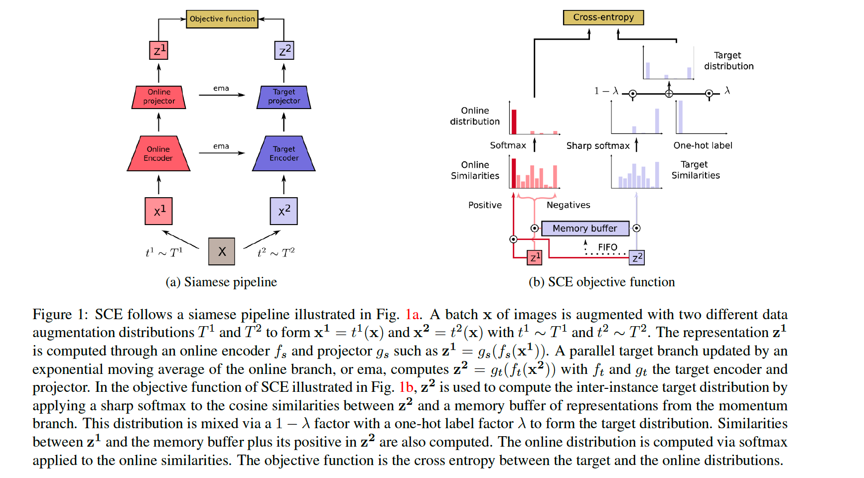
• produce two views of \(\mathrm{x}\)
  • \(\mathrm{x}^1=t^1(\mathrm{x})\) and \(\mathrm{x}^2=\) \(t^2(\mathbf{x})\),
    • from 2 distn \(T^1\) and \(T^2\) ( with \(t^1 \sim T^1\) and \(t^2 \sim T^2\) )
  • \(T^2\) : weak data augmentation distn ( to maintain relations )
• model architecture
  • online network \(f_s\)
  • projector \(g_s\)
• two embeddings ( both are \(l_2\)-normalized. )
  • \(\mathbf{z}^{\mathbf{1}}=g_s\left(f_s\left(\mathbf{x}^{\mathbf{1}}\right)\right)\).
  • \(\mathbf{z}^{\mathbf{2}}=g_t\left(f_t\left(\mathbf{x}^{\mathbf{2}}\right)\right)\). ( model : EMA of online branch )

InfoNCE loss

\(L_{\text {InfoNCE }}=-\frac{1}{N} \sum_{i=1}^N \log \left(\frac{\exp \left(\mathbf{z}_{\mathbf{i}}^1 \cdot \mathbf{z}_{\mathbf{i}}^2 / \tau\right)}{\sum_{j=1}^N \exp \left(\mathbf{z}_{\mathbf{i}}^1 \cdot \mathbf{z}_{\mathbf{j}}^2 / \tau\right)}\right)\).

• a similarity based function
• scaled by the temperature \(\tau\)

ReSSL

target similarity distribution \(\mathbf{s}^{\mathbf{2}}\),

• represents the relations between weak augmented instances
• temperature parameters : \(\tau_m\)

similarity distribution \(\mathbf{s}^{\mathbf{1}}\)

• represents the relations between strong & weak augmented instances
• temperature parameters : \(\tau\) ( where \(\tau>\tau_m\) to eliminate noisy relations )

Loss function :

CE between \(s^2\) and \(s^1\) :

\(\begin{gathered} s_{i k}^1=\frac{\mathbb{1}_{i \neq k} \cdot \exp \left(\mathbf{z}_{\mathbf{i}}^1 \cdot \mathbf{z}_{\mathbf{k}}^2 / \tau\right)}{\sum_{j=1}^N \mathbb{1}_{i \neq j} \cdot \exp \left(\mathbf{z}_{\mathbf{i}}^1 \cdot \mathbf{z}_{\mathbf{j}}^2 / \tau\right)}, \\ s_{i k}^2=\frac{\mathbb{1}_{i \neq k} \cdot \exp \left(\mathbf{z}_{\mathbf{i}}^2 \cdot \mathbf{z}_{\mathbf{k}}^2 / \tau_m\right)}{\sum_{j=1}^N \mathbb{1}_{i \neq j} \cdot \exp \left(\mathbf{z}_{\mathbf{i}}^2 \cdot \mathbf{z}_{\mathbf{j}}^2 / \tau_m\right)}, \\ L_{R e S S L}=-\frac{1}{N} \sum_{i=1}^N \sum_{\substack{k=1 \\ k \neq i}}^N s_{i k}^2 \log \left(s_{i k}^1\right) . \end{gathered}\).

Memory buffer ( size : M » N )

• filled by \(\mathbf{z}^{\mathbf{2}}\)

<br.

(2) SCE (Similarity Contrastive Estimation)

Contrastive Learning

• damage relations among instances which Relational Learning correctly build.

Relational Learning

• lacks the discriminating features that contrastive methods can learn

Similarity Contrastive Estimation (SCE)

We argue that there exists a true distribution of similarity \(\mathbf{w}_{\mathbf{i}}^*\)

• between a query \(\mathbf{q}_{\mathbf{i}}\) and \(\mathbf{x}=\left\{\mathbf{x}_{\mathbf{k}}\right\}_{k \in\{1, \ldots, N\}}\)
  • \(\mathbf{x}_{\mathbf{i}}\) : a positive view of \(\mathbf{q}_{\mathbf{i}}\)

Training framework

• estimate the similarity distribution \(\mathbf{p}_{\mathbf{i}}\)

  • between \(\mathbf{q}_{\mathbf{i}}\) and all instances in \(\mathrm{x}\)

• minimize the CE between \(\mathrm{w}_{\mathbf{i}}^*\) and \(\mathbf{p}_{\mathbf{i}}\)

  = soft contrastive learning objective

Loss Function of SCE

• \(L_{S C E^*}=-\frac{1}{N} \sum_{i=1}^N \sum_{k=1}^N w_{i k}^* \log \left(p_{i k}\right)\).

• SOFT contrastive approach that generalizes InfoNCE and ReSSL objectives

• InfoNCE ( = HARD contrastive loss )
  • estimates a hard contrastive loss that estimates \(\mathrm{w}_{\mathbf{i}}^*\) with a one-hot label
• ReSSL :
  • estimates \(\mathbf{w}_{\mathbf{i}}^*\) without the contrastive component.

This paper : propose an estimation of \(\mathbf{w}_{\mathbf{i}}^*\)

• based on both (1) contrastive and (2) relational learning

• Procedures

  • step 1) \(\mathrm{x}^1=t^1(\mathrm{x})\) & \(\mathrm{x}^2=\) \(t^2(\mathbf{x})\)

  • step 2) \(\mathbf{z}^{\mathbf{1}}=g_s\left(f_s\left(\mathbf{x}^{\mathbf{1}}\right)\right)\) & \(\mathbf{z}^2=g_t\left(f_t\left(\mathbf{x}^2\right)\right) \cdot \mathbf{z}^1\)

    • both are \(l_2\)-normalized

  • step 3) similarity distribution \(\mathbf{s}^2\)

    • \(s_{i k}^2=\frac{\mathbb{1}_{i \neq k} \cdot \exp \left(\mathbf{z}_{\mathbf{i}}^2 \cdot \mathbf{z}_{\mathbf{k}}^2 / \tau_m\right)}{\sum_{j=1}^N \mathbb{1}_{i \neq j} \cdot \exp \left(\mathbf{z}_{\mathbf{i}}^2 \cdot \mathbf{z}_{\mathbf{j}}^2 / \tau_m\right)}\).

  • step 4) build target distn \(\mathbf{w_i}^2\)

    • weighted positive one-hot label is added to \(\mathbf{s_i}^2\)

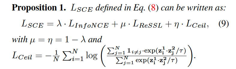
    • \(w_{i k}^2=\lambda \cdot \mathbb{1}_{i=k}+(1-\lambda) \cdot s_{i k}^2\).

  • step 5) compute online similarity distn \(\mathbf{p}_{\mathrm{i}}^1\)
    • between \(\mathbf{z}_{\mathrm{i}}^1\) & \(\mathbf{z}^2\)
    • \(p_{i k}^1=\frac{\exp \left(\mathbf{z}_{\mathbf{i}}^1 \cdot \mathbf{z}_{\mathbf{k}}^2 / \tau\right)}{\sum_{j=1}^N \exp \left(\mathbf{z}_{\mathbf{i}}^1 \cdot \mathbf{z}_{\mathbf{j}}^2 / \tau\right)}\).
  • step 6) objective function : CE loss btw \(\mathbf{w}^2\) & \(\mathbf{p}^1\)
    • \(L_{S C E}=-\frac{1}{N} \sum_{i=1}^N \sum_{k=1}^N w_{i k}^2 \log \left(p_{i k}^1\right)\).

• Memory Buffer :

  • size : \(M >>N\)
  • filled by \(\mathbf{z}^2\)