(paper 70) Contrastive Vicinal Space for Unsupervised Domain Adaptation

Contrastive Vicinal Space for Unsupervised Domain Adaptation

Contents

1. Abstract
2. Introduction
   1. UDA
   2. Consistency Training
3. Methodology
   1. Preliminaries
   2. EMP-Mixup
   3. Contrastive Views and Labels
   4. Label Consensus

0. Abstract

Unsupervised domain adaptation (UDA)

• have utilized ”vicinal” space between source & target domains

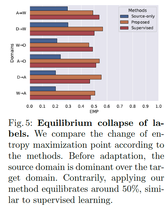
Problem : Equilibrium collapse of labels

• SOURCE labels are dominant over the TARGET labels
• happen in the predictions of vicinal instances

Propose an ”Instance-wise” minimax strategy

• minimizes the entropy of HIGH UNCERTAINTY instances in the vicinal space
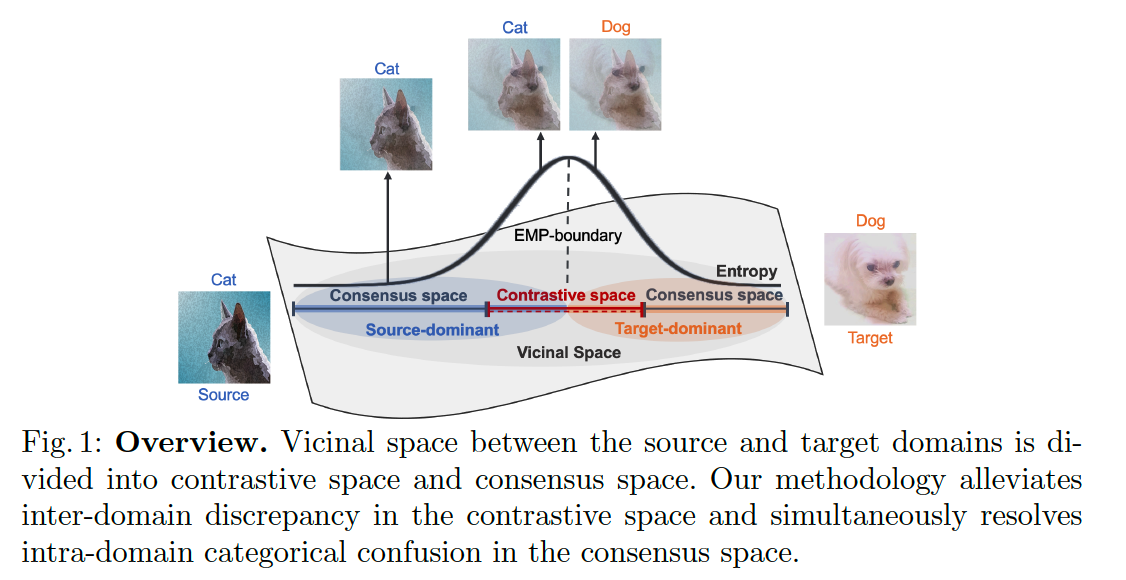
• divide the vicinal space into 2 subspaces
  • (1) contrastive space
    • inter-domain discrepancy is mitigated
    • by constraining instances to have contrastive views and labels
  • (2) consensus space
    • reduces the confusion between intra-domain categories

1. Introduction

(1) UDA (Unsupervised Domain Adaptation)

Idea

• adapt a model trained on (labeled) SOURCE domain
• to (unlabeled) TARGET domain

Problem : domain shift ( distribution shift )

• Arises from the change in data distn ( btw SOURCE & TARGET domain )

Widely used solution :

• leverage intermediate domains btw SOURCE & TARGET
• many approaches have emerged built on data augmentation to construct the intermediate spaces.
  • ex) Mixup augmentation to the DA task
    • use inter-domain mixup to efficiently overcome the domain shift problem by utilizing vicinal instances between the source and target domains

(2) Consistency Training

• one of the promising components for leveraging UN-labeled data
• enforces a model to produce SIMILAR predictions of original & perturbed instances.

Contrastive Vicinal space-based (CoVi) algorithm

• leverages vicinal instances from the perspective of self-training
  • Self-training : approach that uses self-predictions of a model to train itself.

• In vicinal space : SOURCE label is generally dominant over the TARGET label

  • even if vicinal instances consist of a higher proportion of TARGET instances than source instances, their predictions are more likely to be SOURCE labels

  \(\rightarrow\) call this problem : equilibrium collapse of labels between vicinal instances

  ( + entropy of the predictions is maximum at the points where the equilibrium collapse of labels occurs )

Goal : find the point where the entropy is maximized between the vicinal instances

\(\rightarrow\) present EMP-Mixup

<br>

EMP-Mixup

• minimizes the entropy for the entropy maximization point (EMP)
• adaptively adjusts the Mixup ratio
  • according to the combinations of source and target instances
• divide the vicinal space into 2 space
  • (1) SOURCE-dominant & (2) TARGET-dominant
  • using EMP as a boundary (i.e., EMP-boundary)
• vicinal instances of …
  • the SOURCE-dominant space : have source labels as their predicted top-1 label.
  • the TARGET-dominant space : have target labels as their top-1 label

2 specialized subspaces

( to reduce inter-domain & intra-domain discrepancy )

• contrastive space
• consensus space

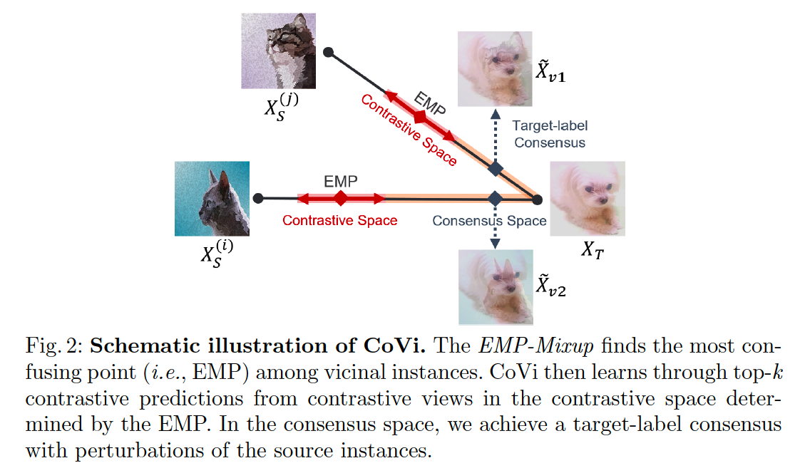
a) CONTRASTIVE space

• to ensure that the vicinal instances have contrastive views :

  • SOURCE-dominant views ( ex. 0.7 source + 0.3 target )
  • TARGET-dominant views ( ex. 0.3 source + 0.7 target )

  \(\rightarrow\) they should have the same top-2 labels containing the source and target labels

• under our constraints, the two contrastive views have opposite order of the first and second labels in the top-2 labels

• propose to impose consistency on predictions of the two contrastive views.

• mitigate INTER_domain discrepancy by solving “swapped prediction” problem

  • predict the top-2 labels of a contrastive view from the other contrastive view.

b) CONSENSUS space

• to alleviate the categorical confusion within the intra-domain
• generate TARGET-dominant vicinal instances
  • utilizing multiple source instances as a perturbation to a single target instance.
    • ex) target 0.7 + source (A) 0.3
    • ex) target 0.7 + source (B) 0.3
  • role of the source instances ( A, B, … )
    • to learn classification information of the source domain (X)
    • to confuse the predictions of the target instances (O)
• can ensure consistent and robust predictions for target instances …
  • by enforcing label consensus among the multiple target-dominant vicinal instances to a single target label

2. Methodology

CoVI introduces 3 techniques

leverage the vicinal space btw SOURCE & TARGET domains

• (1) EMP-Mixup
• (2) Contrastive views & labels
• (3) Label-consensus

(1) Preliminaries

Notation

• \(\mathcal{X}\): mini-batch of \(m\)-images, with labels as \(\mathcal{Y}\)
  • [ SOURCE ] \(\mathcal{X}_{\mathcal{S}} \subset \mathbb{R}^{m \times i}\) and \(\mathcal{Y}_{\mathcal{S}} \subset\) \(\{0,1\}^{m \times n}\)
    • \(n\) : number of classes
    • \(i=c \cdot h \cdot w\).
  • [ TARGET ] \(\mathcal{X}_{\mathcal{T}} \subset \mathbb{R}^{m \times i}\)
• \(\mathcal{Z}\) : extracted features from \(\mathcal{X}\)

Model

consists of the following sub components:

• an encoder \(f_\theta\)
• a classifier \(h_\theta\)
• an EMP-learner \(g_\phi\)

Mixup

Mixup based on the Vicinal Risk Minimization (VRM)

• virtual instances constructed with the linear interpolation of 2 instances

Define the inter-domain Mixup applied between the source and target domains as …

• \(\tilde{\mathcal{X}}_\lambda=\lambda \cdot \mathcal{X}_{\mathcal{S}}+(1-\lambda) \cdot \mathcal{X}_{\mathcal{T}}\).
• \(\tilde{\mathcal{Y}}_\lambda=\lambda \cdot \mathcal{Y}_{\mathcal{S}}+(1-\lambda) \cdot \hat{\mathcal{Y}}_{\mathcal{T}}\).
  • \(\hat{\mathcal{Y}}_{\mathcal{T}}\) : pseudo labels of the target instances

Empirical risk for vicinal instances : \(\mathcal{R}_\lambda=\frac{1}{m} \sum_{i=1}^m \mathcal{H}\left[h\left(f\left(\tilde{\mathcal{X}}_\lambda^{(i)}\right)\right), \tilde{\mathcal{Y}}_\lambda^{(i)}\right]\).

(2) EMP-Mixup

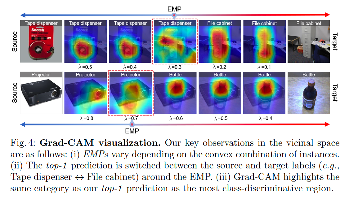
2 observiations in the vicinal space

• Observation 1. “The labels of the TARGET domain are relatively recessive to the SOURCE domain labels.”
• Observation 2. “Depending on the convex combinations of source and target instances, the label dominance is changed.”

Observation 1

• investigate the dominance of the predicted top-1 labels between the source and target instances in vicinal instances.
• find that the label dominance is balanced, when the labels of both the source and target domains are provided
  • top-1 label = determined by the instance with larger proportion.
• UDA : un-labeled ( the label of the target domain is not given )
  • Balance of label dominance is broken (i.e., equilibrium collapse of labels).
  • discover that source labels frequently represent vicinal instances even with a higher proportion of target instances than source instances.

Observation 2

• label dominance is altered according to the convex combinations of instances
  • implies that an instance-wise approach can be a key to solving the label equilibrium collapse problem
• discover that the entropy of the prediction is maximum at the point where the label dominance changes
  • because the source and target instances become most confusing at this point
• aim to capture and mitigate the most confusing points
  • vary with the combination of instances
• introduce a minimax strategy to break through the worst-case risk among the vicinal instances

MinMax Strategy

• minimize the worst risk by finding the entropy maximization point (EMP) among the vicinal instances.

• to estimate the EMPs, we introduce a small network, \(E M P\)-learner \(g_\phi\)

  • aims to generate Mixup ratios that maximize the entropy of the encoder \(f_\theta\) followed by a classifier \(h_\theta\).

Procedure

• step 1) instance features

  • \(\mathcal{Z}_{\mathcal{S}}=f_\theta\left(\mathcal{X}_{\mathcal{S}}\right)\) & \(\mathcal{Z}_{\mathcal{T}}=f_\theta\left(\mathcal{X}_{\mathcal{T}}\right)\)

• step 2) concatenate

  • pass the concatenated features \(\mathcal{Z}_{\mathcal{S}} \oplus \mathcal{Z}_{\mathcal{T}}\) to \(g_\phi\).

• step 3) produces the entropy maximization ratio \(\lambda^*\)

  • maximizes the entropy of the \(f_\theta\)
  • Mixup ratios for our EMP-Mixup :
    • \(\lambda^*=\underset{\lambda \in[0,1]}{\arg \max } \mathcal{H}\left[h_\theta\left(f_\theta\left(\tilde{\mathcal{X}}_\lambda\right)\right)\right]\), where \(\lambda=g_\phi\left(\mathcal{Z}_{\mathcal{S}} \oplus \mathcal{Z}_{\mathcal{T}}\right)\).

• step 4) objective function for EMP-learner

  • maximize the entropy :

    • \(\mathcal{R}_\lambda(\phi)=\frac{1}{m} \sum_{i=1}^m \mathcal{H}\left[h\left(f\left(\tilde{\mathcal{X}}_\lambda^{(i)}\right)\right)\right]\).

  • only update the parameter \(\phi\) of the EMP-learner

    ( not \(\theta\) of the encoder and the classifier )

• step 5) EMP-Mixup minimizes the worst-case risk ( on vicinal instances )

  • \[\mathcal{R}_{\lambda^*}(\theta)=\frac{1}{m} \sum_{i=1}^m \mathcal{H}\left[h\left(f\left(\tilde{\mathcal{X}}_{\lambda^*}^{(i)}\right)\right), \tilde{\mathcal{Y}}_{\lambda^*}^{(i)}\right]\]

• \(\lambda^*=\left[\lambda_1, \ldots, \lambda_m\right]\) : has different optimized ratios

• Overall objective functions : \(\mathcal{R}_{e m p}=\mathcal{R}_{\lambda^*}(\theta)-\mathcal{R}_\lambda(\phi)\)

(3) Contrastive Views and Labels

Observation 3

“The dominant/recessive labels of the vicinal instances are switched at the EMP.”

with the EMP as a boundary (i.e., EMP-boundary)…

• the dominant/recessive label is switched between the source and target domains

  = vicinal instances around the EMP-boundary should have source and target labels as their top-2 labels.

• divide the vicinal space into …

  • (1) source-dominant space
  • (2) target-dominant space

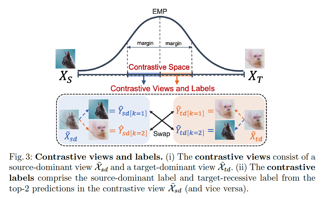
source-dominant space

• \(\lambda^*-\omega<\lambda_{s d}<\lambda^*\).

target-dominant space

• \(\lambda^*<\lambda_{t d}<\lambda^*+\omega\).
  • \(\omega\) : margin of the ratio from the EMP-boundary

source-dominant instances \(\tilde{\mathcal{X}}_{s d}\) &target dominant instances \(\tilde{\mathcal{X}}_{t d}\) have contrastive views of each other.

focus on the top- 2 labels for each prediction

• only interested in the classes that correspond to the source and target instances, not the other classes.
• define a set of top-2 one-hot labels within a mini-batch as \(\hat{\mathcal{Y}}_{[k=1]}\) and \(\hat{\mathcal{Y}}_{[k=2]}\).

Labels for the instances

• of TARGET-dominant space : \(\hat{\mathcal{Y}}_{t d}=\lambda_{t d} \cdot \hat{\mathcal{Y}}_{t d[k=1]}+\left(1-\lambda_{t d}\right) \cdot \hat{\mathcal{Y}}_{t d[k=2]}\)

• of SOURCE-dominant space : \(\hat{\mathcal{Y}}_{s d}=\lambda_{s d} \cdot \hat{\mathcal{Y}}_{s d[k=1]}+\left(1-\lambda_{s d}\right) \cdot \hat{\mathcal{Y}}_{s d[k=2]}\)

propose a new concept of contrastive labels

• constrain the top-2 labels from the contrastive views as follows:

  • \(\hat{\mathcal{Y}}_{s d[k=1]}\) from \(\tilde{\mathcal{X}}_{s d}\) and \(\hat{\mathcal{Y}}_{t d[k=2]}\) from \(\tilde{\mathcal{X}}_{t d}\) must be equal, as the predictions of the SOURCE instances.

  • \(\hat{\mathcal{Y}}_{s d[k=2]}\) must be equal to \(\hat{\mathcal{Y}}_{t d[k=1]}\), as for the predictions of the TARGET instances.

solve a “swapped” prediction problem

• enforce consistency to the top-2 contrastive labels obtained from contrastive views of the same source and target instance combinations.

Final objective for our contrastive loss

( in target-dominant space )

• \(\mathcal{R}_{t d}(\theta)=\frac{1}{m} \sum_{i=1}^m \mathcal{H}\left[h\left(f\left(\tilde{\mathcal{X}}_{t d}^{(i)}\right)\right), \hat{\mathcal{Y}}_{t d}^{(i)}\right]\).
  • where \(\hat{\mathcal{Y}}_{t d}=\lambda_{t d} \cdot \hat{\mathcal{Y}}_{s d[k=2]}+\left(1-\lambda_{t d}\right) \cdot \hat{\mathcal{Y}}_{s d[k=1]}\).

( in source-dominant space )

• vise vera

\(\rightarrow\) \(\mathcal{R}_{ct} = \mathcal{R}_{t d}(\theta) + \mathcal{R}_{s d}(\theta)\)

(4) Label Consensus

Contrastive & Consensus Space

• contrastive space ) confusion between the source and target instances is crucial
• consensus space ) focus on uncertainty of predictions within the intra-domain than inter-domain instances

Consensus Space

• exploit multiple source instances to impose perturbations to target predictions

  ( rather than classification information for the source domain )

• makes a model more robust to the target predictions

  • by enforcing consistent predictions on the target instances even with the source perturbations.

Target-label consensus

step 1) Construct 2 randomly shuffled versions of the source instances within a mini-batch

step 2) Apply Mixup with a single target mini-batch

• obtain two different perturbed views \(v_1\) and \(v_2\)
• mixup ratio = sufficiently small
  • since too strong perturbations can impair the target class semantics

step 3) Compute two softmax probabilities from the perturbed instances \(\tilde{\mathcal{X}}_{v_1}\) and \(\tilde{\mathcal{X}}_{v_2}\)

• using an encoder & classifier

step 4) Aggregate the softmax probabilities &yield a one-hot prediction \(\hat{\mathcal{Y}}\).

Assign the label \(\hat{\mathcal{Y}}\) to both versions of the perturbed target-dominant instances \(\tilde{\mathcal{X}}_{v_1}\) and \(\tilde{\mathcal{X}}_{v_2}\).

Imposing consistency to differently perturbed instances for a single target label

= allows us to focus on categorical information for the target domain

Objective for label consensus

\(\mathcal{R}_{c s}(\theta)=\frac{1}{m} \sum_{i=1}^m\left[\mathcal{H}\left(h\left(f\left(\tilde{\mathcal{X}}_{v_1}^{(i)}\right), \hat{\mathcal{Y}}^{(i)}\right)\right)+\mathcal{H}\left(h\left(f\left(\tilde{\mathcal{X}}_{v_2}^{(i)}\right), \hat{\mathcal{Y}}^{(i)}\right)\right)\right]\).

• where \(\mathcal{H}\) is the cross-entropy loss.