
Layer Grafted Pretraining; Briding Contrastive Learning and Masked Image Modeling for Label-Efficient Representations
Contents
- Abstract
- Introduction
- Related Work
0. Abstract
CL & MIM : powerful to learn good representations
\(\rightarrow\) However, naively combining them is far from success.
Empirical observation that a naive joint optimization of CL and MIM losses leads to conflicting gradient directions ( more severe as the layers go deeper )
\(\rightarrow\) choose proper learning method per network layer
Find that MIM and CL are suitable to lower and higher layers, respectively
\(\rightarrow\) propose to combine them in simple way, “sequential cascade” ( Layer Grafted Pre-training )
- early layers : first trained under one MIM loss, on top of which latter layers continue to be trained under another CL loss.
1. Introduction
CL & MIM : follow different mechanisms & manifest different strengths
- CL : instance-level task
- MIM : draws inspiration from BERT & performs masked token or pixel reconstruction
- facilitates the learning of rich local structures within the same image
\(\rightarrow\) Although MIM has recently surpassed CL on the fine-tuning performance of many datasets, CL often remains to be a top competitor in data-scarce few-shot downstream applications
Q) CL and MIM indeed complementary to each other, and is there a way to best combine their strengths?
- simple way : multiple task learning (MTL) & jointly optimize the two losses
\(\rightarrow\) such a vanilla combination FAILS to improve over either baseline
( often compromising the single loss’s performance )
Q) If the two losses conflict when both are placed at the end, how about placing them differently, such as appending them to different layers?
- (Experimental observations)
- Lower layers : learn better from the MIM loss
- ( in order to capture local spatial details )
- Higher layers : benefit more from the CL loss
- ( in order to learn semantically-aware grouping and invariance )
\(\rightarrow\) propose a simple MIM → CL Grafting idea to combine the bests of both worlds
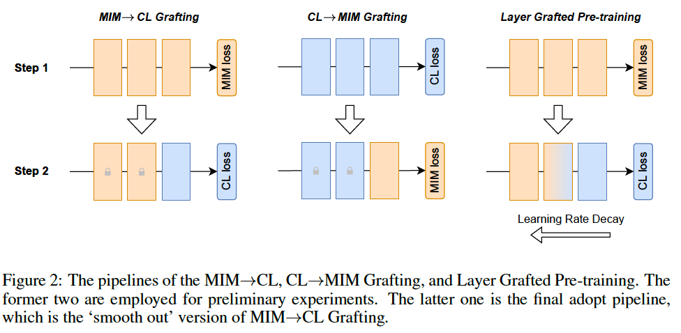
Layer Grafted Pre-training
- step 1) train lower layers with MIM loss & fixing their weights
- step 2) train higher layer with CL loss
\(\rightarrow\) This simple cascaded training idea neatly separates MIM and CL losses to avoid their conflicts !!
- “‘smooth out” the grafting by allowing lower layers to be slowly tuned in step 2
Ablation experiments : the order of grafting matters!
- reversing MIM/CL loss locations and performing CL→MIM will considerably damage the performance.
Contribution
- propose Layer Grafted Pre-training
- principled framework to merge MIM and CL,
- investigate the different preferences of lower and higher layers towards CL and MIM losses, and show the order of grafting to matter.
2. Method
(1) Preliminary and Overview
a) CL
\(\mathcal{M}\left(v_i, v_i^{+}, V^{-}, \tau\right)=\frac{1}{N} \sum_{i=1}^N-\log \frac{\exp \left(v_i \cdot v_i^{+} / \tau\right)}{\exp \left(v_i \cdot v_i^{+} / \tau\right)+\sum_{v_i^{-} \in V^{-}} \exp \left(v_i \cdot v_i^{-} / \tau\right)}\).
- \(V^{-}\): pool of negative features
- \(N\) : number of samples
b) MIM
\(\mathcal{L}\left(x_i, M\right)=\frac{1}{N} \sum_{i=1}^N D\left(d\left(f\left(M x_i\right)\right), x_i\right)\).
Overview
- 2-2) preliminary exploration on the MTL of MIM and CL tasks
- reveals the existence of the conflicting gradient direction.
- 2-3) provide a simple separating idea towards mitigating the conflicts
- 2-4) Layer Grafted Pre-training
(2) Conflicts Prevent MTL from working
( Simple Idea ) Multi-Task Learning (MTL) combination
- composed of two steps.
- step 1) images are augmented twice for computing the CL loss
- step 2) image with minimal augmentation would be utilized for computing MIM loss following MAE
- two losses share the same encoder
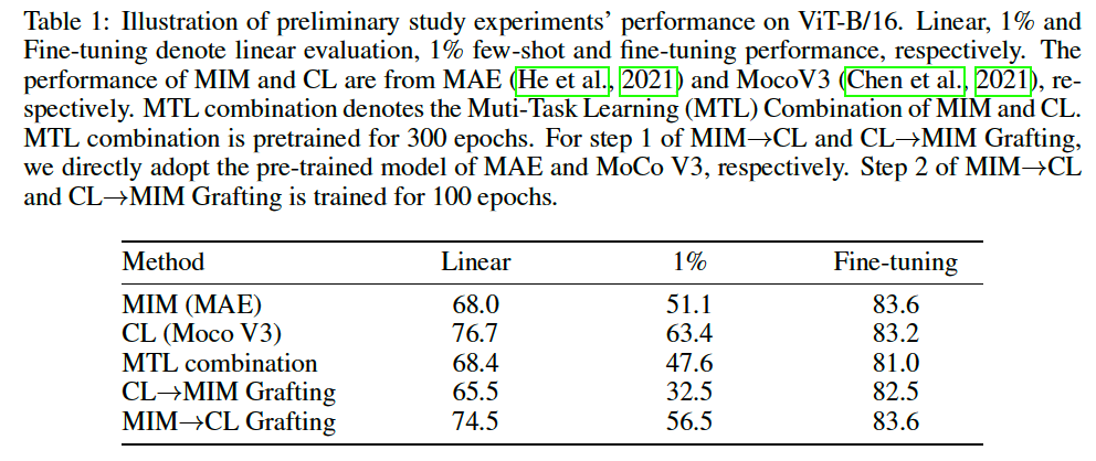
- MTL only yields a marginal performance improvement of \(0.4 \%\) on linear evaluation compared to the MIM baseline ( 68.0 < 68.4)
- still much lower that the CL baseline ( 76.7 > 68.4)
- on both \(1 \%\) few-shot and fine-tuning : even inferior
MTL combination is the cause of the bad performance !
To verify it, we design a gradient surgery experiment by computing the cosine similarity between gradients of two tasks
\(\mathbf{C}_{\mathrm{MIM}, \mathrm{CL}}(x)=\frac{\nabla_\theta L_{\mathrm{MIM}}(x)^T}{ \mid \mid \nabla_\theta L_{\mathrm{MIM}}(x) \mid \mid } \frac{\nabla_\theta L_{\mathrm{CL}}(x)}{ \mid \mid \nabla_\theta L_{\mathrm{CL}}(x) \mid \mid }\).
- (Figure 1) measure the distribution of \(\mathrm{C}_{\mathrm{MIM}, \mathrm{CL}}(x)\) across different layers of a pre-trained MTL model
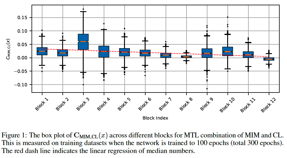
Findings
-
(1) always exist negative values for \(\mathrm{C}_{\mathrm{MIM}, \mathrm{CL}}(x)\),
( = where the \(\mathrm{MIM}\) and \(\mathrm{CL}\) are optimized in opposite directions )
-
(2) gradient direction varies across layers
( + more severe as layers go deeper )
Also, the conflicts can be reflected in two losses’ contradictory targets to enforce.
-
(1) MIM loss : requires that the reconstruction have the same brightness, color distribution, and positions as the input image
\(\rightarrow\) \(\therefore\) the model needs to be sensitive to all these augmentations.
-
(2) CL loss : designed to ensure that the model remains invariant regardless of different augmentations
(3) Addressing the Conflicts via Separating
Question ) If the two losses conflict …. how about placing them differently ?
- ex) such as appending them to differen layers?
\(\rightarrow\) Recent empirical evidence suggests that CL and MIM may favor different pre-training methods.
[MIM] Wang et al. (2022c)
When only the pre-trained lower layers are retained ( while the higher layers are reset to random initialization ), most of the gain is still preserved for downstream fine-tuning tasks.
\(\rightarrow\) Lower layers appear to be a key element in MIM
[CL] Chen et al. (2021)
Ineffective and even unstable for training the projection layer ( = the earliest/lower layer of ViT )
- Fixing its weight to be random initialization can even yield significantly higher performance!
\(\rightarrow\) CL excels at semantic concepts, which happen often at higher layers of the neural network.
Propose a simple MIM→CL Grafting framework ( two steps )
- step 1) lower layers are first trained with MIM and then fixed
- step 2) higher layers continue to learn with CL
\(\rightarrow\) yields promising preliminary results as shown in Table 1
What if reverse order? ( = CL→MIM Grafting )
-
suffer a dramatic drop in performance
( = which is even lower than the MTL combination )
Huge gap between CL→MIM and MIM→CL Grafting further confirms the preference of MIM and CL towards lower and higher layers, respectively.
(4) Layer Grafted Pre-training
To fully unleash the power of Grafting, we ‘smooth out’ the boundary of MIM→CL grafting to avoid a sudden change in the feature space.
\(\rightarrow\) rather than fixing the lower layers, we assign them a small learning rate
( = termed as Layer Grafted Pre-training )