(paper 75) SimTS; Rethinking Contrastive Representation Learning for Time Series Forecasting

SimTS: Rethinking Contrastive Representation Learning for Time Series Forecasting

Contents

1. Abstract
2. Introduction
   1. Problems of CL in TS
   2. SimTS
   3. Contribution
3. Methods
   1. Notation
   2. Four parts of SimTS
   3. Process
   4. Multi-scale Encoder
   5. Stop-gradient
   6. Final Loss

0. Abstract

Contrastive learning in TS

Problem (1)

• GOOD for TS classification
• BAD for TS forecasting … Reason?
  • Optimization of instance discrimination is not directly applicable to predicting the future state from the history context.

Problem (2)

• Construction of positive and negative pairs strongly relies on specific time series characteristics

\(\rightarrow\) restricting their generalization across diverse types of time series data

Proposal : SimTS ( = simple representation learning approach for improving time series forecasting )

• by learning to predict the future from the past in the latent space
• does not rely on negative pairs or specific assumptions about the characteristics of TS

1. Introduction

(1) Problems of CL in TS

Problem 1) Bad for TSF

Mostly rely on instance discrimination

• can discriminate well between different instances of TS ( good for TSC )
• but features learned by instance discrimination may not be sufficient for TSF

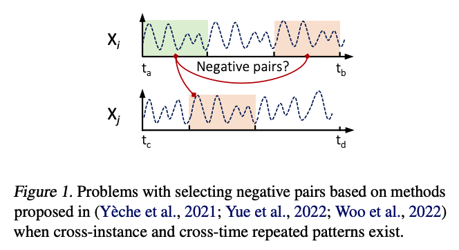
Problem 2) Defining POS & NEG

identifying positive and negative pairs for time series forecasting is challenging

• previous works : several assumptions

  • (1) the similarity between segments of the same time series decreases as the time lag increases
  • (2) segments of distinctive time series are dissimilar

  \(\rightarrow\) However, particular time series do not adhere to these assumptions

  • ex) TS with seasonality??

(2) SimTS

aims to answer the following key question:

Q1) “What is important for TSF with CL, and how can we adapt contrastive ideas more effectively to TSF tasks?”

• Beyond CL, propose Simple Representation Learning Framework for Time Series Forecasting (SimTS)

  • inspired by predictive coding
  • learn a representation such that the latent representation of the future time windows can be predicted from the latent representation of the history time windows
  • build upon a siamese network structure

• Details : propose key refinements

  • (1) divide a given TS into history and future segments

  • (2) ENCODER : map to latent space

  • (3) PREDICTIVE layer : predict the latent representation of the future segment from the history segment.

    • ( predicted representation & encoded representation ) = positive pairs

      \(\rightarrow\) representations learned in this way encode features that are useful for forecasting tasks.

Q2) Questions existing assumptions and techniques used for constructing POS & NEG pairs.

• detailed discussion and several experiments showing their shortcomings

  • ex) question the idea of augmentation

• SimTS does not use negative pairs to avoid false repulsion

• hypothesize that the most important mechanism behind representation learning for TSF

  = maximizing the shared information between representations of history and future time windows.

(3) Contribution

(1) propose a novel method (SimTS) for TSF

• employs a siamese structure and a simple convolutional encoder
• learn representations in latent space without requiring negative pairs

(2) Experiments on multiple types of benchmark datasets.

• SOTA Our method outperforms state-of-the-art methods for multivariate time series forecasting

  ( BUT still worse than Supervised TSF models & MTM )

(3) extensive ablation experiments

2. Methods

(1) Notation

• input TS : \(X=\left[x_1, x_2, \ldots, x_T\right] \in \mathbb{R}^{C \times T}\),
  • \(C\) : the number of features (i.e., variables)
  • \(T\) : the sequence length
• Segmented subTS
  • history segment : \(X^h=\left[x_1, x_2, \ldots, x_K\right]\), where \(0<K<T\),
  • future segment : \(X^f=\left[x_{K+1}, x_{K+2}, \ldots, x_T\right]\)
• Encoder : \(F_\theta\)
  • maps historical and future segments to their corresponding latent representations
  • learn an informative latent representation \(Z^h=F_\theta\left(X^h\right)=\left[z_1^h, z_2^h, \ldots, z_K^h\right] \in \mathbb{R}^{C^{\prime} \times K}\)
    • will be used to predict the latent representation of the future through a prediction network

(2) Four parts of SimTS

Objective : learns time series representations by maximizing the similarity between ..

• (1) predicted latent features
• (2) encoded latent features

for each timestamp.

( Consists of FOUR main parts )

(1) Siamese network

• consists of two identical networks that share parameters.

• TS is divided into the (a) history segment \(X^h\) & (b) future segment \(X^f\)

  \(\rightarrow\) given as inputs to the siamese network.

• learns to map them to their latent representations \(Z^h, Z^f\).

(2) Multi-scale encoder

• consist of a projection layer
• projects raw features into a high dimensional space and multiple CNN blocks with different kernel sizes.

(3) Predictor network \(G_\phi\)

• takes the last column of the encoded history view as input and predicts the future in latent space.

(4) Cosine similarity loss

• considers only positive samples

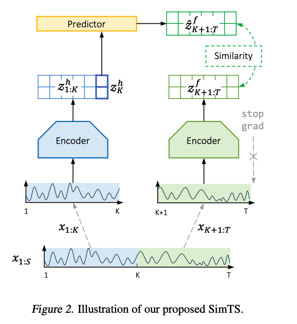
(3) Process

Encoding

• History encoding : \(Z^h=F_\theta\left(X^h\right)\)

• Future encoding : \(Z^f=F_\theta\left(X^f\right)=\left[z_{K+1}^f, z_{K+2}^f, \ldots, z_T^f\right] \in \mathbb{R}^{C^{\prime} \times(T-K)}\)

Prediction

• use predictior network \(G_\phi\) ( = MLP ) on the last column of \(Z^h\) ( = \(z_K^h\) )
• to predict the future latent representations: \(\hat{Z}^f=G_\phi\left(z_K^h\right)=\left[\hat{z}_{K+1}^f, \hat{z}_{K+2}^f, \ldots, \hat{z}_T^f\right] \in \mathbb{R}^{C^{\prime} \times(T-K)}\).
  • last column : allows the encoder to condense the history information into a summary by properly choosing the kernel size.
• positive pair = ( \(Z^f\), \(\hat{Z}^f\) )
• calculate the negative cosine similarity between them
  • \(\operatorname{Sim}\left(\hat{Z}^f, Z^f\right)=-\frac{1}{T-K} \sum_{i=K+1}^T \frac{\hat{z}_i^f}{ \mid \mid \hat{z}_i^f \mid \mid _2} \cdot \frac{z_i^f}{ \mid \mid z_i^f \mid \mid _2}\).

(4) Multi-scale Encoder

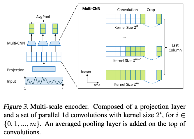
Structure of \(F_\theta\) plays a vital role!

• Should extract temporal dependency from local ~ global patterns
  • for SHORT-term forecasting : local patterns
  • for LONG-term forecasting : global patterns
• thus, propose to use CNN with multiple kernel sizes ( of total \(m\) )

Details of \(F_\theta\) :

• Step 1) each TS is passed through CNN projection layer

• Step 2) for a time series \(X\) with length \(K\), we have \(m=\left[\log _2 K\right]+1\) parallel CNN layers on the top of the projection layer
  • \(i\) th convolution has kernel size \(2^i\), where \(i \in\{0,1, \ldots, m\}\).
  • each convolution \(i\) takes the latent features from the projection layer and generates a representation \(\hat{Z}_{(i)}\).
• Step 3) Averaging
  • the final multi-scale representation \(Z\) are obtained by averaging across \(\hat{Z}_{(0)}, \hat{Z}_{(1)}, \ldots, \hat{Z}_{(m)}\).

(5) Stop-gradient

• stop-gradient operation to the future encoding path

• As the encoder should constrain the latent of the past to be predictive of the latent of the future ..

  \(\rightarrow\) only \(\hat{Z}^f\) can only move towards \(Z^f\) in the latent space,

(6) Final Loss

( for one sample \(X=\left[X^h, X^f\right]\) )

\(\begin{aligned} \mathcal{L}_{\theta, \phi}\left(X^h, X^f\right) & =\operatorname{Sim}\left(G_\phi\left(F_\theta\left(X^h\right)\right), F_{\mathrm{sg}(\theta)}\left(X^f\right)\right) \\ & =\operatorname{Sim}\left(\hat{Z}^f, \operatorname{sg}\left(Z^f\right)\right) \end{aligned}\).

( Loss for a mini-batch \(\mathcal{D}=\left\{X_i^h, X_i^f\right\}_{i \in[1: N]}\) )

\(\mathcal{L}_{\theta, \phi}(\mathcal{D})=\frac{1}{N} \sum_{i=1}^N \mathcal{L}_{\theta, \phi}\left(X_i^h, X_i^f\right)\).