Contrastive Mixup : Self- and Semi-Supervised Learning for Tabular Domain
Contents
- Abstract
- Preliminaries
- Self-SL
- Semi-SL
- Method : Contrastive Mixup
- Semi-Self SL for Tabular Data
- Pseudo-labeling Unlabeled Samples
- Predictor
0. Abstract
propose Contrastive Mixup
- SSL in tabular domain
- effective in limited annotated data settings
Details:
- leverages Mixup-based augmentation
- encourage interpolated samples to have high similarity within the same labeled class
- unlabeled samples : employed via a transductive label propagation
1. Preliminaries
formulate the self- & semi-supervised problem
Notation :
- dataset with \(N\) examples ( \(\mid \mathcal{D}_L \mid \ll \mid \mathcal{D}_U \mid )\)
- (1) labeled : \(\mathcal{D}_L=\left\{\left(x_i, y_i\right)\right\}_{i=1}^{N_L}\)
- (2) unlabeled : \(\mathcal{D}_U=\left\{\left(x_i\right)\right\}_{i=1}^{N_U}\)
- \(x_i \sim p(x)\) , \(y_i \in\{0,1, \cdots, c\}\)
- classifier : \(f: \mathcal{X} \rightarrow \mathcal{Y} \in \mathcal{F}\)
- \(f=\min _{f \in \mathcal{F}} \sum_{i=1}^N l_A\left(f\left(x_i\right), y_i\right)\).
(1) Self-Supervised Learning
a) pre-text tasks
- ex) in-painting, rotation, jig-saw
b) contrastive learning
- learning a batch of \(N\) samples is augmented through an augmentation function
- create a multi-viewed batch with \(2 N\) pairs, \(\left\{\tilde{x}_i, \tilde{y}_i\right\}_{i=1 \cdots 2 N}\)
- \(z=e(x)\) : samples are fed to an encoder \(e: x \rightarrow z\)
- minimize a self-supervised loss function \(l_{s s}\).
- \(\min _{e, h} \mathbb{E}_{(x, \tilde{y}) \sim P(X, \tilde{Y})}[l(\tilde{y}, h \circ e(x)]\)….where \(h: z \rightarrow v\)
Within multi-viewed batch…
- \(i \in \mathcal{I}=\{1, \cdots 2 N\}\).
- SSL loss : \(l=\sum_{i \in \mathcal{I}}-\log \left(\frac{\exp \left(\operatorname{sim}\left(v_i, v_{j(i)}\right) / \tau\right)}{\sum_{n \in \mathcal{I} \backslash\{i\}} \exp \left(\operatorname{sim}\left(v_i, v_n\right) / \tau\right)}\right)\)
- \(\mathcal{A}(i)\) : positives
- \(\mathcal{I} \backslash\{i\}\) : negatives
(2) Semi-Supervised learning
predictive model \(f\) is optimized to minimize a supervised loss, jointly with an unsupervised loss
- \(\min _f \mathbb{E}_{(x, y) \sim P(X, Y)}[l(y, f(x))]+\beta \mathbb{E}_{\left(x, y_{p s}\right) \sim P\left(X, Y_{p s}\right)}\left[l_u\left(y_{p s}, f(x)\right)\right]\).
- term 1) estimated over \(\mathcal{D}_U\)
- term 2) estimated over \(\mathcal{D}_L\)
Unsupervised loss function \(l_u\) :
- to help the downstream prediction task
- ex) consistency loss training, supervised objective on pseudo-labeled samples
2. Method : Contrastive Mixup
Contrative Mixup
- semi-supervised method for multimodal tabular data
-
propose semi-supervised training to learn an encoder
-
propose to train a classifier using the pre-trained encoder and pseudo-labels
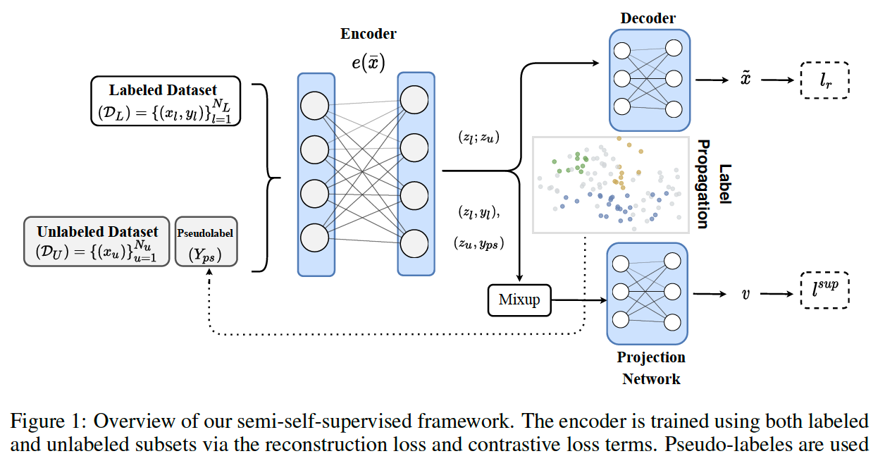
(1) Semi-Self-Supervised Learning for Tabular Data
Data : mutli-modal tabular data rows \(x_i \in \Re^d\) = concatenation of …
- (1) discrete features \(D=\left[D_1, \cdots, D_{ \mid D \mid }\right]\)
- (2) continuous features \(\mathcal{C}=\left[C_1, \cdots, C_{ \mid \mathcal{C} \mid }\right]\)
step 1) \(x_i \in \Re^d\) are fed to embedding layer ( \(E : x \rightarrow \bar{x}\) )
step 2) \(\bar{x} \in Re^{ \mid C \mid +\sum_i^{ \mid D \mid } d_{ \mid \mathcal{D}_i \mid }}\) are fed to encoder
- \(z = e(\bar{x})\).
step 3) fed to feature estimation pre-text task
- semi-supervised contrastive loss
Tabular Domain
how to augment data ?
\(\rightarrow\) propose to interpolate between samples of the same class
ex) given labeled examples \(\mathcal{D}_{\mathcal{B}}=\left\{x_k, y_k\right\}_{k=1}^K\)
- new labeled sample : \((\hat{x}, \hat{y})\)
- \(\hat{x}=\lambda x_1+(1-\lambda) x_2\).
- \(\lambda \sim \mathcal{U}(0, \alpha)\) with \(\alpha \in[0,0.5]\)
- \(y_1=y_2=\hat{y}\).
- \(\hat{x}=\lambda x_1+(1-\lambda) x_2\).
Applying Mixup in the input space ?
\(\rightarrow\) may lead to low probable samples due to the multi-modality of the data & presence of categorical columns
Instead, we map samples to the hidden space and interpolate there.
( encoder : \(f_t\) ( where \(t\in {1, \cdots, T}\) ) )
- \(\tilde{h}_{12}^t=\lambda h_1^t+(1-\lambda) h_2^t\).
Then, pass \(\tilde{h}_{i^{\prime} i}^t\) through the rest of the encoder layers & obtain \(z\) !
- \(z_l\) : labeled samples
- \(z_u\) : unlabeled samples
( we only consider the labeled portion for the contrastive term )
Loss function
- (1) supervised contrastive loss for \(\mathcal{D}_L\) as augmentation views
- \(l_\tau^{s u p}=\sum_{i \in \mathcal{I}} \frac{-1}{P(i)} \sum_{p \in P(i)} \log \left(\frac{\exp \left(\operatorname{sim}\left(h_i^{\text {proj }}, h_p^{\text {proj }}\right) / \tau\right)}{\sum_{n \in N e(i)} \exp \left(\operatorname{sim}\left(h_i^{\text {proj}}, h_n^{\text {proj }}\right) / \tau\right)}\right)\).
- \(P(i)=\left\{p \mid p \in \mathcal{A}(i), y_i=\tilde{y}_p\right\}\).
- \(\mid P(i) \mid\) : cardinality
- \(N e(i)=\left\{n \mid n \in \mathcal{I}, y_i \neq y_n\right\}\).
- \(l_\tau^{s u p}=\sum_{i \in \mathcal{I}} \frac{-1}{P(i)} \sum_{p \in P(i)} \log \left(\frac{\exp \left(\operatorname{sim}\left(h_i^{\text {proj }}, h_p^{\text {proj }}\right) / \tau\right)}{\sum_{n \in N e(i)} \exp \left(\operatorname{sim}\left(h_i^{\text {proj}}, h_n^{\text {proj }}\right) / \tau\right)}\right)\).
- (2) feature reconstruction loss ( via decoder \(f_{\theta}(\cdot)\) )
- \(l_r\left(x_i\right)=\frac{ \mid C \mid }{d} \sum_c^{ \mid C \mid } \mid \mid f_\theta \circ e_\phi\left(x_i\right)^c-x_i^c \ \mid _2^2+\frac{ \mid D \mid }{d} \sum_j^{ \mid D \mid } \sum_o^{d_{D_j}} 1\left[x_i^d=o\right] \log \left(f_\theta \circ e_\phi\left(x_i\right)^o\right)\).
Final Loss function :
- \(L=\mathbb{E}_{(x, y) \sim \mathcal{D}_L}\left[l_\tau^{s u p}(y, f(x))\right]+\beta \mathbb{E}_{x \sim \mathcal{D}_U \cup \mathcal{D}_L}\left[l_r(x)\right]\).
(2) Pseudo-labeling Unlabeled Samples
to use \(\mathcal{D}_U\), propose using label propagation
( after \(K\) epochs of training with the supervised contrastive loss )
After some training with \(\mathcal{D}_L\) ….
- map \(\mathcal{D}_L\) & \(S_U \subset \mathcal{D}_U\) to the latent space \(z_l\)
- then, construct affinity matrix \(G\)
\(g_{i j}:= \begin{cases}\operatorname{sim}\left(z_i, z_j\right) & \text { if } i \neq j \text { and } z_j \in \mathrm{NN}_k(i) \\ 0 & \text { otherwise }\end{cases}\).
Then obtain pseudo labels for \(S_U\) by …
- step 1) compute the diffusion matrix \(C\)
- \((I-\alpha \mathcal{A}) C=Y\).
- (adjacency matrix) \(\mathcal{A}=D^{-1 / 2} W D^{-1 / 2}\).
- \(W=G^T+G\).
- \(D:=\operatorname{diag}\left(W 1_n\right)\).
- (adjacency matrix) \(\mathcal{A}=D^{-1 / 2} W D^{-1 / 2}\).
- \((I-\alpha \mathcal{A}) C=Y\).
- step 2) \(\tilde{y}_i:=\arg \max _j c_{i j}\)
After obtaining pseudo-labels….
\(\rightarrow\) train the encoder with unlabeled samples ( + pseudo-labels )
\(L=\mathbb{E}_{(x, y) \sim \mathcal{D}_L}\left[l^{s u p}(y, f(x))\right]+\gamma \mathbb{E}_{\left.\left(x, y_{p s}\right) \sim S_U\right)}\left[l^{s u p}\left(y_{p s}, f(x)\right)\right]+\beta \mathbb{E}_{x \sim \mathcal{D}_U}\left[l_r(x)\right]\).
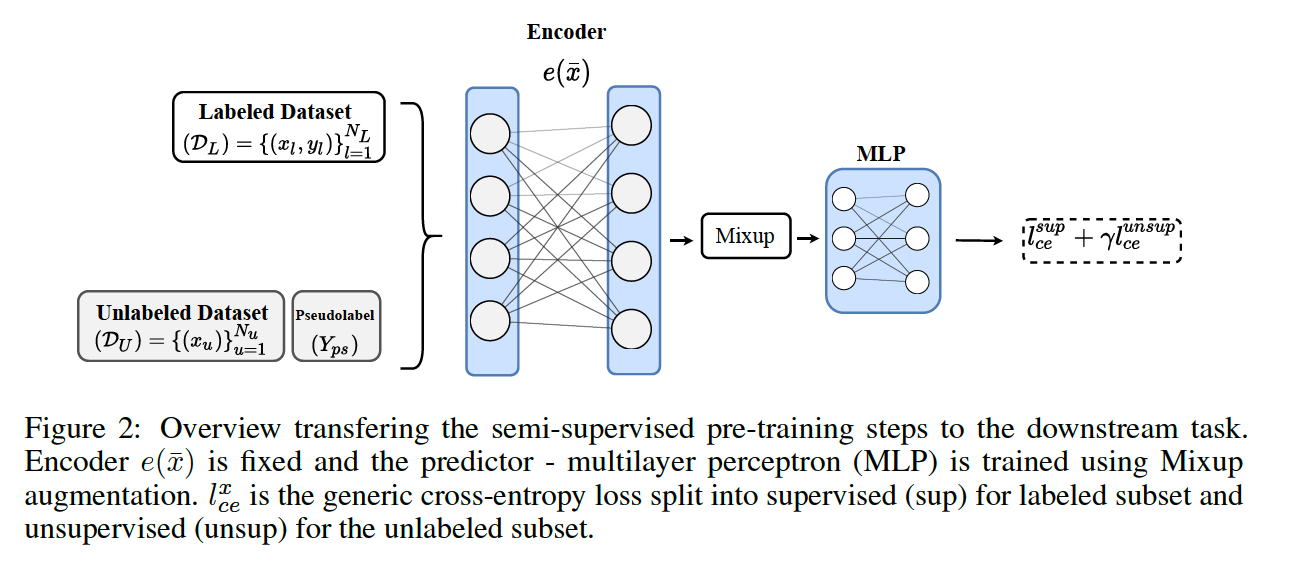
(3) Predictor
encoder is transferred to the downstream task, with generated pseudo-labels
to train the predictor of downstream task