
Self-Supervised TS Representation Learning with Temporal-Instance Similarity Distillation
Contents
- Abstract
- Introduction
- Related Work
- Method
- Problem Definition
- Model Architecture
- Loss function
0. Abstract
propose SSL method for pretraining universal TS
- learn contrastive representations,
- using similarity distillation along the “temporal” and “instance” dimensions
3 downstream tasks
- TS classification
- TS forecasting
- Anomaly detection
1. Introduction
-
leverage similarity distillation
( as an alternative source of self-supervision to traditional negative-positive contrastive pairs )
-
propose to learn contrastive representations using **similarity distillation
- along the temporal and instance dimensions.
2. Related Work
pre-training approaches in TS
-
(old) seq2seq architecture
-
(new) pretext tasks
examples :
- TST : learning the masked values in TST (Zerveas et al., 2021)
- TS-TCC : contrastive learning on different augmentations of the input series (Eldele et al., 2021)
- T-Loss (Franceschi et al., 2019)
- TNC (Tonekaboni et al., 2021)
- TS2Vec (Yue et al., 2022)
Contrastive methods :
-
shown to have a better performance
-
trained by augmenting every batch
However…. Contrastive methods
-
rely on the assumption that the augmentation of a given sample will generate a negative pair with other samples in the batch
\(\rightarrow\) not always valid!!
Solution : ( instead of using pos & neg pairs with contrastive learning ) use knowledge distillation based approaches
- student network is trained to produce the same similarity PDF as a teacher network
- has never been used for pre-training TS representations
3. Method
(1) Problem Definition
- Time Series : \(\mathcal{X}=\left\{x^1, x^2, \ldots, x^N\right\}\)
- # of TS : \(N\)
- each TS : \(x^i\) ( with \(T_i\) timestamps )
- Representation of \(x^i\) : \(\mathbf{r}^i=\left\{\mathbf{r}_1^i, \mathbf{r}_2^i, \ldots, \mathbf{r}_{T_i}^i\right\}\)
- each \(\mathbf{r}_j^i \in \mathbb{R}^d\) : representation of TS \(i\) at timestamp \(j\)
(2) Model Architecture
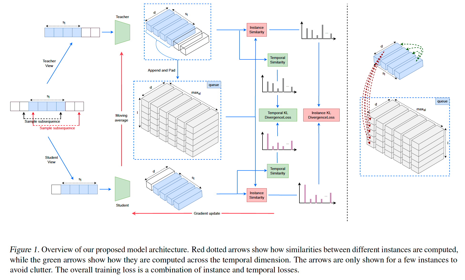
student-teacher framework that uses similarity distillation
a) Data Augmentation technique ( as TS2Vec )
- sample two overlapping subsequences from the same sequence.
- These two are applied to a teacher & student
- gradient : only to student
- teacher = MA of student
b) Student & Teacher ( as TS2Vec ) : consists of 3 components
- (1) input projection layer
-
(2) timestamp masking module
- (3) dilated CNN module.
c) Similarity Distillation
-
first to leverage in TS data
-
applying the student & teacher to the subsequences :
\(\rightarrow\) results in \(s_l \times d\) matrices ( \(s_l\) : length of overlap )
d) Memory Buffer ( as a queue )
-
to store a set of anchor sequences
-
teacher representations in the overlapping region are appended
\(\rightarrow\) \(l \times \text{max}s_l \times d\) matrix of anchor representations
- \(l\) : length of the buffer
- max\(s_l\) : max overlap length ( use zero-padding )
e) Goal
capture the …
- (1) temporal objective :
- relationship between the events at various timestamps within the same sequence
- (2) instance objective :
- relationship across different sequences
f) Notation
\(\mathbf{s}_j\) : student representation of augmented sequence at temporal position \(j\)
\(\mathbf{t}_j\) : teacher representation ~
(3) Loss function
a) Temporal Loss :
step 1-1) contrast \(\mathbf{s}_j\) with the other student representations of the same augmented sequence, at all other temporal positions (green dotted arrows)
- \(s_l\) -dim pdf : \(\mathbf{p}_{s, j}^{\text {temp }}(k)=\frac{\exp \left(\operatorname{sim}\left(\mathbf{s}_j, \mathbf{s}_k\right) / \tau\right)}{\sum_{m=1}^{s_l} \exp \left(\operatorname{sim}\left(\mathbf{s}_j, \mathbf{s}_m\right) / \tau\right)}\)
step 1-2) contrast \(\mathbf{t}_j\) ~
- \(s_l\) -dim pdf : \(\mathbf{p}_{t, j}^{\text {temp }}(k)=\frac{\exp \left(\operatorname{sim}\left(\mathbf{t}_j, \mathbf{t}_k\right) / \tau\right)}{\sum_{m=1}^{s_l} \exp \left(\operatorname{sim}\left(\mathbf{t}_j, \mathbf{t}_m\right) / \tau\right)}\).
Temporal Loss : summing the KL divergences \(K L\left(\mathbf{p}_{t, j}^{\text {temp }}, \mathbf{p}_{s, j}^{\text {temp }}\right)\) over all temporal positions
- \(\mathcal{L}^{\text {temp }}=\sum_{j=1}^{s_l} K L\left(\mathbf{p}_{t, j}^{\text {temp }} \mid \mid \mathbf{p}_{s, j}^{\text {temp }}\right)\).
b) Instance Loss
- contrasts \(\mathbf{s}_j\) with the representations of buffered sequences at temporal position \(j\) (red dotted arrows)
- \(l\)-dim student pdf : \(\mathbf{p}_{s, j}^{\text {inst }}(k)=\frac{\exp \left(\operatorname{sim}\left(\mathbf{s}_j, \mathbf{q}_j^k\right) / \tau\right)}{\sum_{m=1}^l \exp \left(\operatorname{sim}\left(\mathbf{s}_j, \mathbf{q}_j^m\right) / \tau\right)}\)
- \(l\)-dim teacher pdf : \(\mathbf{p}_{t, j}^{\text {inst }}(k)=\frac{\exp \left(\operatorname{sim}\left(\mathbf{t}_j, \mathbf{q}_j^k\right) / \tau\right)}{\sum_{m=1}^l \exp \left(\operatorname{sim}\left(\mathbf{t}_j, \mathbf{q}_j^m\right) / \tau\right)}\)
- \(\mathbf{q}^k\) : \(k\) th anchor sequence in the memory buffer
Instance Loss : summing the KL divergences \(K L\left(\mathbf{p}_t^{\text {inst }} \mid \mid \mathbf{p}_s^{\text {inst }}\right)\) over all temporal positions
- \(\mathcal{L}^{\text {inst }}=\sum_{j=1}^{s_l} K L\left(\mathbf{p}_{t, j}^{\text {inst }} \mid \mid \mathbf{p}_{s, j}^{\text {inst }}\right)\).
c) overall SSL loss
\(\mathcal{L}=\alpha \cdot \mathcal{L}^{\text {inst }}+(1-\alpha) \cdot \mathcal{L}^{\text {temp }}\).