Context Understanding - Visual Transformer

( 참고 : 패스트 캠퍼스 , 한번에 끝내는 컴퓨터비전 초격차 패키지 )

Context Understanding - Visual Transformer

Contents

1. Stand-alone self-attention
2. Vision Transformer (ViT)
3. Visual Transformer (VT)
4. DeiT
5. ConViT
6. CeiT
7. Swin Transformer
8. T2T-ViT
9. PVT
10. Vision Transformers with patch diversification

1. Stand-alone self-attention

( Ramachandran, Prajit, et al. “Stand-alone self-attention in vision models.” Advances in Neural Information Processing Systems 32 (2019). )

• https://arxiv.org/abs/1906.05909

(1) Stand-alone self-attention

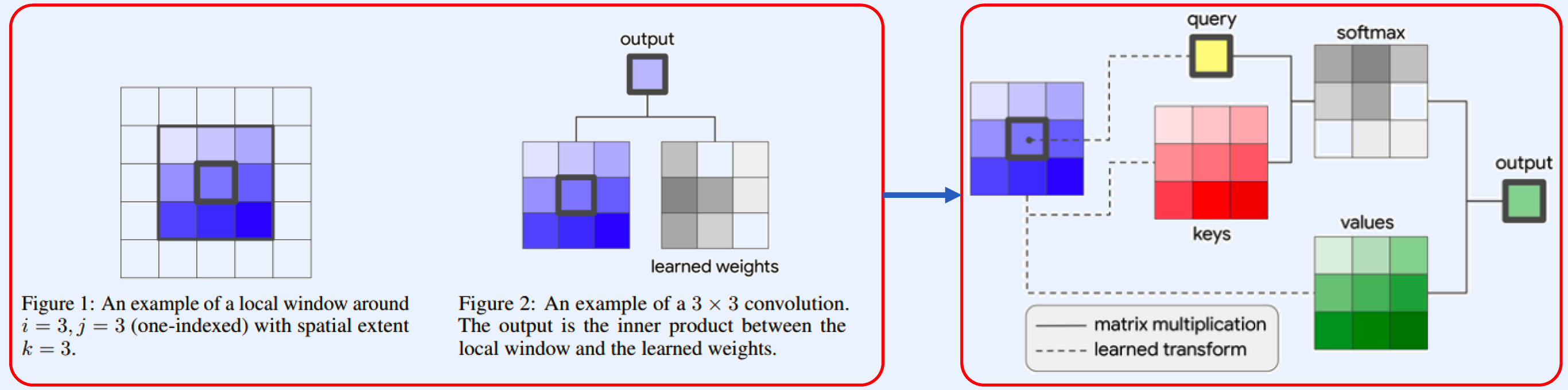
• (LEFT) standard CNN
• (RIGHT) stand-alone self-attention

\(y_{i j}=\sum_{a, b \in \mathcal{N}_{k}(i, j)} \operatorname{softmax}_{a b}\left(q_{i j}^{\top} k_{a b}\right) v_{a b}\).

• (Q) \(q_{i j}=W_{Q} x_{i j}\).
• (K) \(k_{a b}=W_{K} x_{a b}\).
• (V) \(v_{a b}=W_{V} x_{a b}\).

\(\operatorname{softmax}_{a b}\) : softmax applied to all logits computed in the neighborhood of \(i j\).

(2) Relative Distance

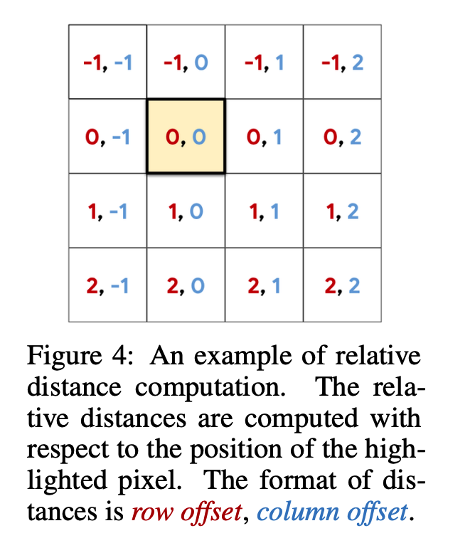
\(y_{i j}=\sum_{a, b \in \mathcal{N}_{k}(i, j)} \operatorname{softmax} \operatorname{tm}_{a b}\left(q_{i j}^{\top} k_{a b}+q_{i j}^{\top} r_{a-i, b-j}\right) v_{a b}\).

2. Vision Transformer (ViT)

( Dosovitskiy, Alexey, et al. “An image is worth 16x16 words: Transformers for image recognition at scale.” arXiv preprint arXiv:2010.11929 (2020). )

• https://arxiv.org/abs/2010.11929

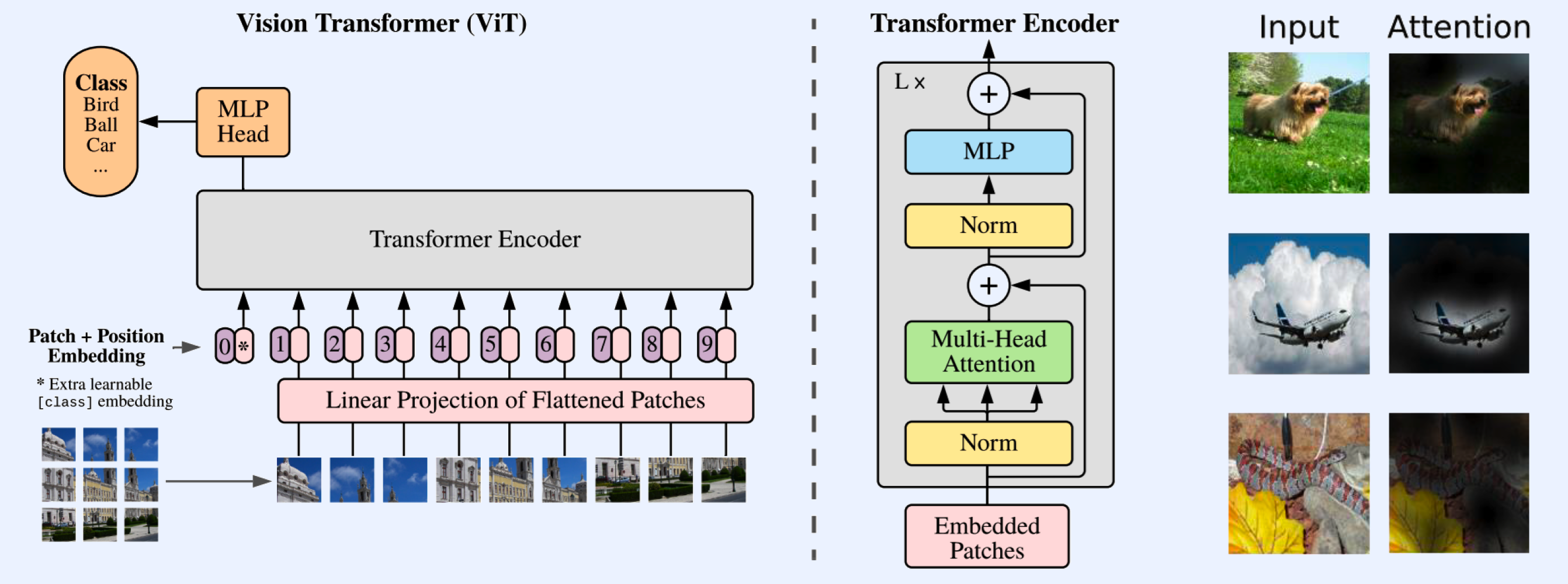
https://seunghan96.github.io/cv/vision_09_ViT/

3. Visual Transformer (VT)

( Wu, Bichen, et al. “Visual transformers: Token-based image representation and processing for computer vision.” arXiv preprint arXiv:2006.03677 (2020). )

• https://arxiv.org/pdf/2006.03677.pdf

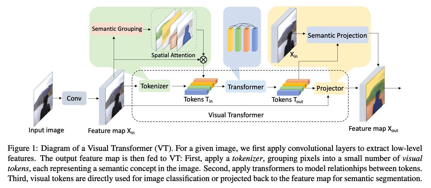
(1) Tokenizer

• (Intuition) Image = summary of words (=visual tokens)
• use tokneizer to convert
  • feature maps \(\rightarrow\) compact sets of visual tokens
• ex)
  • a) Filter-based Tokenizer
  • b) Recurrent Tokenizer

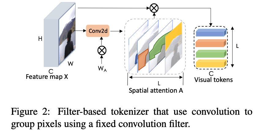
a) Filter-based Tokenizer

Notation

• feature map : \(\mathbf{X}\)
• each pixel : \(\mathbf{X}_{p} \in \mathbb{R}^{C}\)
  • map each pixel to one of \(L\) semantic groups, using point-wise convolution

Wihtin each group… spatially pool pixels to obtain tokens \(\mathbf{T}\)

• \(\mathbf{T}=\underbrace{\operatorname{softmax}_{H W}\left(\mathbf{X} \mathbf{W}_{A}\right)^{T}}_{\mathbf{A} \in \mathbb{R}^{H W \times L}} \mathbf{X}\).

  • \(\mathbf{W}_{A} \in \mathbb{R}^{C \times L}\) : forms semantic groups from \(\mathbf{X}\)

• computes weighted averages of pixels in \(\mathbf{X}\) to make \(L\) visual tokens.

  ( weighted average matrix : \(\mathbf{A}\) )

b) Recurrent Tokenizer

• recurrent tokenizer with weights that are dependent on previous layer’s visual tokens

• incrementally refine the set of visual tokens, conditioned on previously-processed concepts

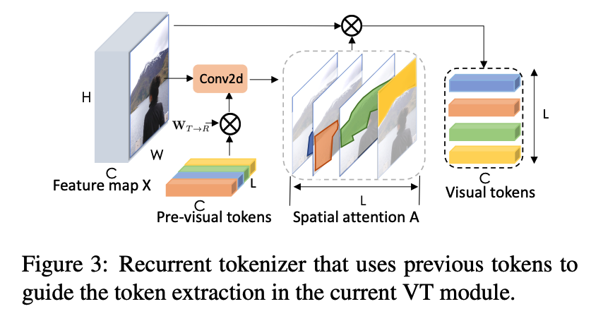
\(\mathbf{W}_{R}=\mathbf{T}_{i n} \mathbf{W}_{\mathbf{T} \rightarrow \mathbf{R}}\).

\[\mathbf{T}=\operatorname{SOFTMAX}_{H W}\left(\mathbf{X} \mathbf{W}_{R}\right)^{T} \mathbf{X}\]

• where \(\mathbf{W}_{T \rightarrow R} \in \mathbb{R}^{C \times C}\)

(2) Projector

Many vision tasks require pixel-level details

\(\rightarrow\) not preserved in visual tokens!

\(\rightarrow\) fuse the transformer’s output with the feature map

\(\mathbf{X}_{o u t}=\mathbf{X}_{i n}+\operatorname{SOFTMAX}_{L}\left(\left(\mathbf{X}_{i n} \mathbf{W}_{Q}\right)\left(\mathbf{T W}_{K}\right)^{T}\right) \mathbf{T}\),

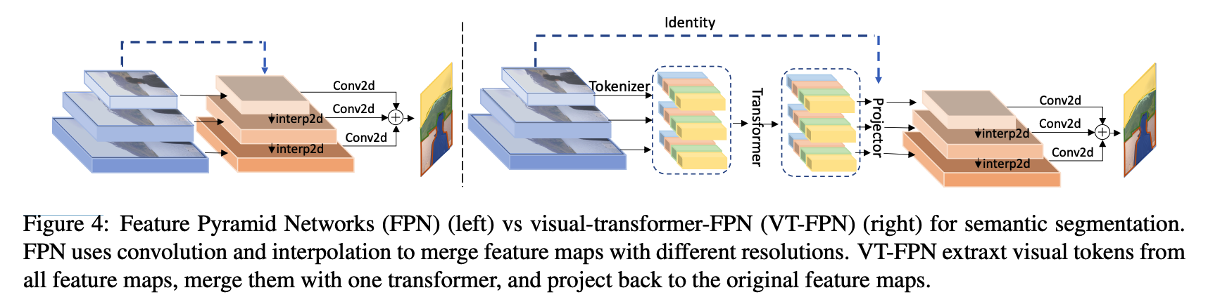
(3) VT for semantic segmentation

4. DeiT

( Touvron, Hugo, et al. “Training data-efficient image transformers & distillation through attention.” International Conference on Machine Learning. PMLR, 2021. )

• https://arxiv.org/abs/2012.12877

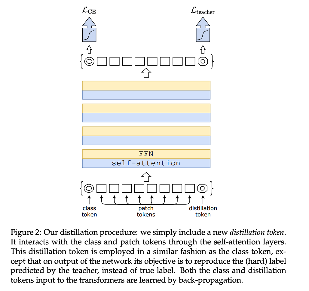
Add distillation token!

• CNN vs Transformer

  • CNN : good for locality

  \(\rightarrow\) learn locality from CNN, by treating them as a teacher model

5. ConViT

( d’Ascoli, Stéphane, et al. “Convit: Improving vision transformers with soft convolutional inductive biases.” International Conference on Machine Learning. PMLR, 2021. )

• https://arxiv.org/abs/2103.10697

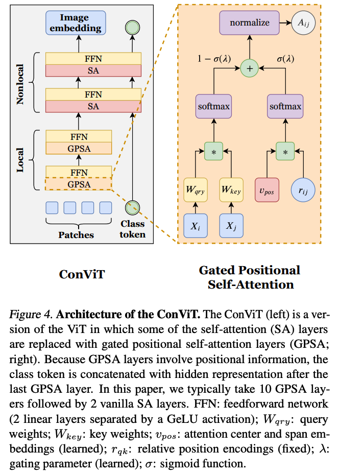
SA (Self-Attention) layer is replaced with GPSA (Gated Positional Self-Attention) layer

(1) GPSA (Gated Positional Self-Attention) layer

• contains positional information

\(\begin{aligned} \operatorname{GPSA}_{h}(\boldsymbol{X}):=& \text { normalize }\left[\boldsymbol{A}^{h}\right] \boldsymbol{X} \boldsymbol{W}_{\text {val }}^{h} \\ \boldsymbol{A}_{i j}^{h}:=&\left(1-\sigma\left(\lambda_{h}\right)\right) \operatorname{softmax}\left(\boldsymbol{Q}_{i}^{h} \boldsymbol{K}_{j}^{h \top}\right) +\sigma\left(\lambda_{h}\right) \operatorname{softmax}\left(\boldsymbol{v}_{p o s}^{h \top} \boldsymbol{r}_{i j}\right) \end{aligned}\).

6. CeiT

( Yuan, Kun, et al. “Incorporating convolution designs into visual transformers.” Proceedings of the IEEE/CVF International Conference on Computer Vision. 2021. )

• https://arxiv.org/pdf/2103.11816.pdf

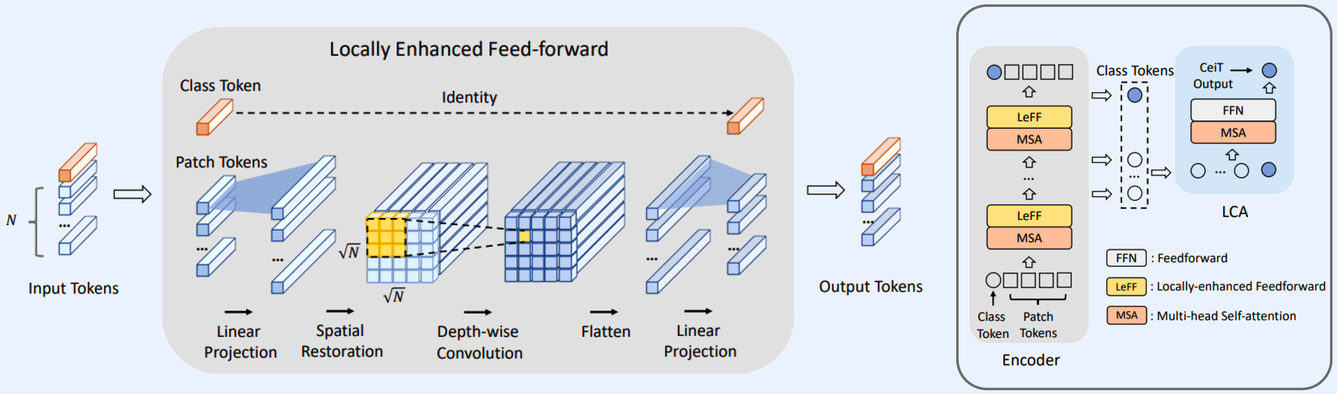
Step 1) tokenize inputs ( = patch tokens )

Step 2) project path tokens to higher dimensions

Step 3) back to original position ( keep spatial info )

Step 4) depth-wise Conv

Step 5) flatten & project to initial dimension

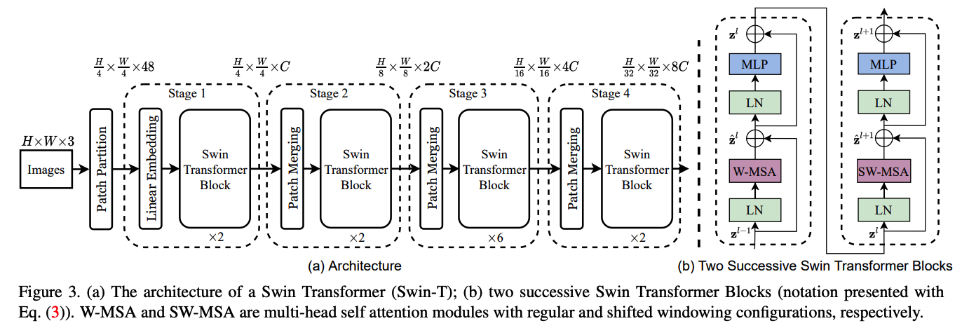
7. Swin Transformer

( Liu, Ze, et al. “Swin transformer: Hierarchical vision transformer using shifted windows.” Proceedings of the IEEE/CVF International Conference on Computer Vision. 2021. )

• https://arxiv.org/abs/2103.14030

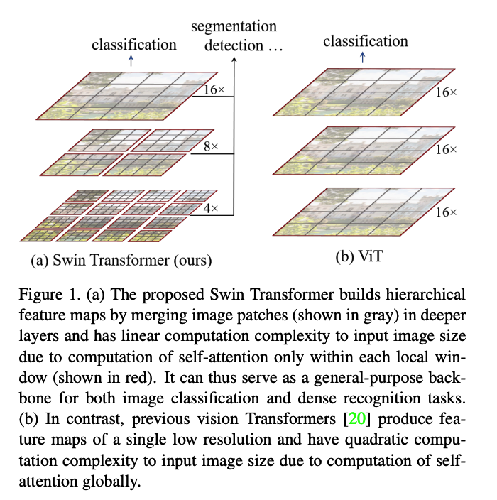
Shift the window in the next layer!

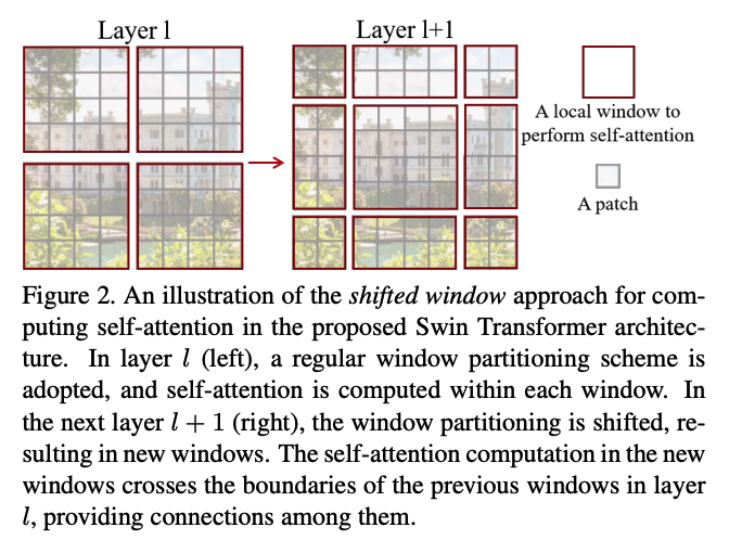
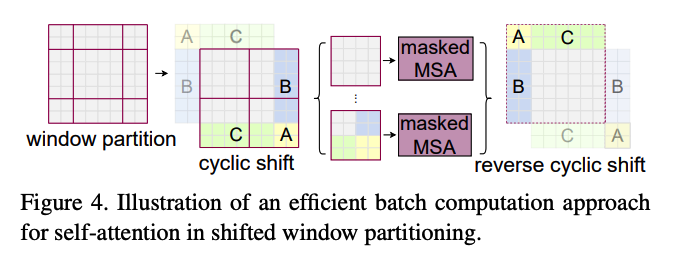
Using the Swin Transformer Block…

8. T2T-ViT

( Yuan, Li, et al. “Tokens-to-token vit: Training vision transformers from scratch on imagenet.” Proceedings of the IEEE/CVF International Conference on Computer Vision. 2021. )

• https://arxiv.org/pdf/2101.11986.pdf

Tokens-to-Token ViT ( T2T-ViT )

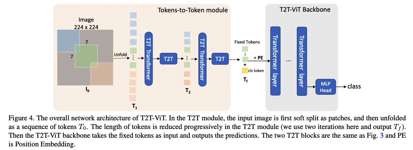
Share some tokens, when generating the next token!!

( = overlapping token )

T2T process

(1) Re-structurization

• (transformation) \(T^{\prime}=\operatorname{MLP}(\operatorname{MSA}(T))\)
• (reshape) \(I=\operatorname{Reshape}\left(T^{\prime}\right)\)

(2) Soft-Split

• length of output tokens \(T_0\) : \(l_{o}=\left\lfloor\frac{h+2 p-k}{k-s}+1\right\rfloor \times\left\lfloor\frac{w+2 p-k}{k-s}+1\right\rfloor\)

(3) T2T module

\(\begin{aligned} &T_{i}^{\prime}=\operatorname{MLP}\left(\operatorname{MSA}\left(T_{i}\right),\right. \\ &I_{i}=\operatorname{Reshape}\left(T_{i}^{\prime}\right), \\ &T_{i+1}=\operatorname{SS}\left(I_{i}\right), \quad i=1 \ldots(n-1) . \end{aligned}\).

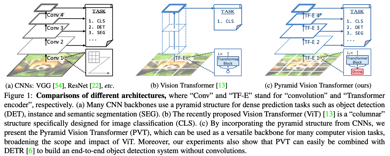
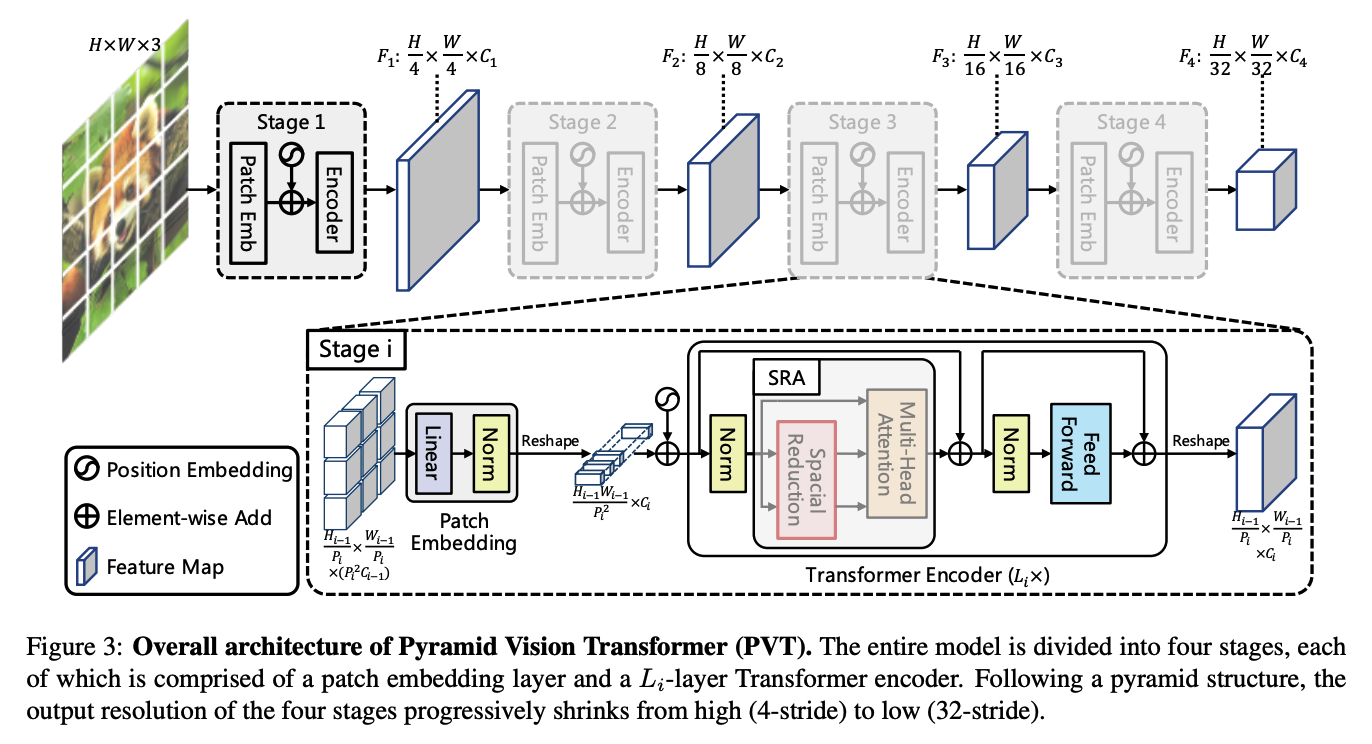
9. PVT (Pyramid Vision Transformer )

( Wang, Wenhai, et al. “Pyramid vision transformer: A versatile backbone for dense prediction without convolutions.” Proceedings of the IEEE/CVF International Conference on Computer Vision. 2021. )

• https://arxiv.org/abs/2102.12122

(1) Pyramid Structure

(2) SRA (Spatial Reduction Attention)

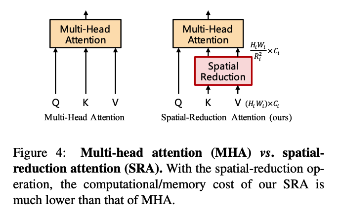
\(\operatorname{SRA}(Q, K, V)=\operatorname{Concat}\left(\operatorname{head}_{0}, \ldots, \operatorname{head}_{N_{i}}\right) W^{O}\).

• \(\operatorname{head}_{j}=\text { Attention }\left(Q W_{j}^{Q}, \mathrm{SR}(K) W_{j}^{K}, \mathrm{SR}(V) W_{j}^{V}\right)\).
  • \(\operatorname{SR}(\mathbf{x})=\operatorname{Norm}\left(\operatorname{Reshape}\left(\mathbf{x}, R_{i}\right) W^{S}\right)\).

(3) Overall Structure

10. Vision Transformers with patch diversification

( Gong, Chengyue, et al. “Vision transformers with patch diversification.” arXiv preprint arXiv:2104.12753 (2021). )

• https://arxiv.org/abs/2104.12753

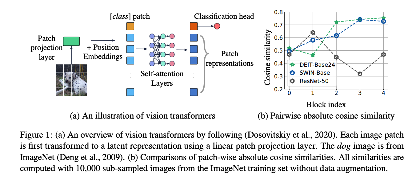
TOO DEEP layers

\(\rightarrow\) over smotthing ( not much difference between the patches ! )

( = No patch diversity :( )

• patch-wise absolute cosine similarity : \(\mathcal{P}(\boldsymbol{h})=\frac{1}{n(n-1)} \sum_{i \neq j} \frac{ \mid h_{i}^{\top} h_{j} \mid }{ \mid \mid h_{i} \mid \mid _{2} \mid \mid h_{j} \mid \mid _{2}}\).

DiversePatch

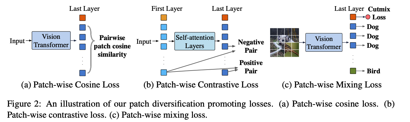
\(\rightarrow\) promote patch diversification for ViT

• (1) Patch-wise cosine loss
  • \(\mathcal{L}_{\cos }(\boldsymbol{x})=\mathcal{P}\left(\boldsymbol{h}^{[L]}\right)\).
• (2) patch-wise contrastive loss
  • \(\mathcal{L}_{\text {contrastive }}(\boldsymbol{x})=-\frac{1}{n} \sum_{i=1}^{n} \log \frac{\exp \left(h_{i}^{[1]^{\top}} h_{i}^{[L]}\right)}{\exp \left(h_{i}^{[1]^{\top}} h_{i}^{[L]}\right)+\exp \left(h_{i}^{[1]^{\top}}\left(\frac{1}{n-1} \sum_{j \neq i} h_{j}^{[L]}\right)\right)}\).
• (3) patch-wise mixing loss
  • \(\mathcal{L}_{\text {mixing }}(\boldsymbol{x})=\frac{1}{n} \sum_{i=1}^{n} \mathcal{L}_{c e}\left(g\left(h_{i}^{[L]}\right), y_{i}\right)\).

Final Loss : weighted combination

• \(\alpha_{1} \mathcal{L}_{\text {cos }}+\alpha_{2} \mathcal{L}_{\text {contrastive }}+\alpha_{3} \mathcal{L}_{\text {mixing }}\).