(paper 55) TF-C

Self-Supervised Contrastive Pre-Training For TS via Time-Frequency Consistency

Contents

1. Abstract
2. Introduction
3. Related Work
   1. Pre-training for TS
   2. Contrastive Learning with TS
4. Problem FOrmulation
5. Our Approach
   1. Time-based Contrastive Encoder
   2. Frequency-based Contrastive Encoder
   3. Time-Frequency Consistency
   4. Implementation and Technical Details

0. Abstract

Pre-training in TS domain :

• need to accommodate target domains with different temporal dynamics

Expect that time-based and frequency-based representations of the same example :

\(\rightarrow\) located close together in the time frequency space

Time-Frequency Consistency (TF-C)

embedding a time-based neighborhood of a particular example

close to its frequency-based neighborhood

\(\rightarrow\) desirable for pre-training.

Define a decomposable pre-training model

• self-supervised signal is provided by the distance between time & frequency components
• each individually trained by contrastive estimation.

1. Introduction

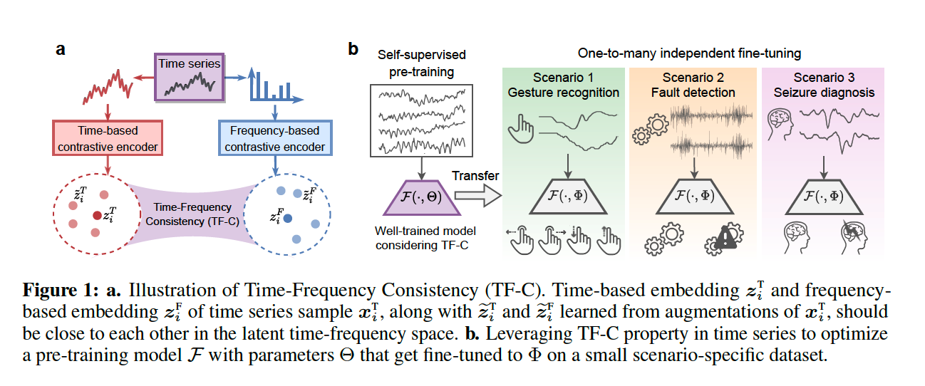
introduce a strategy for SSL pre-training in TS, by modeling Time-Frequency Consistency (TF-C)

TF-C

Definition : time-based representation & frequency-based representation are…

• closer to each other in a joint time-frequency space ( if from same TS )
• farther apart ~ ( if from different TS )

Details :

• adopts contrastive learning in time space to generate a time-based representation

• propose a set of novel augmentations

  • based on the characteristic of frequency spectrum

    \(\rightarrow\) produce a frequency-based embedding through contrastive instance discrimination

  ( first work that implements augmentation in frequency domain )

• pre-training objective :

  • minimize the distance between the time-based & frequency-based embeddings
  • with dedicated consistency loss

2. Related Work

(1) Pre-training for TS

SSL pre-training for TS remains underexplored

Shi et al. [11]

• developed the only model to date that is explicitly designed for SSL TS pre-training
• captures the local and global temporal pattern
• not convincing why the designed pretext task can capture generalizable representations.

proposed : TF-C

• designed to be invariant to different TS datasets
• does not need any labels during pre-training
• can produce generalizable pre-training models

(2) Contrastive Learning with TS

CL in TS is less investigated

• due to the challenge of identifying augmentations that capture key invariance properties in TS data.

Examples 1 )

• CLOCS : adjacent segments of a TS as positive pairs
• TNC : overlapping neighborhoods of TS should be similar

\(\rightarrow\) both leverage temporal invariance to define positive pairs

Examples 2) other invariances :

• transformation invariance (SimCLR)
• contextual invariance (TS2vec, TS-TCC)

Example 3) CoST

• processes sequential signals through frequency domain

  but the augmentations are still implemented in time space

TF-C

Propose an augmentation bank that exploits multiple invariances to generate diverse augmentations

• propose ”frequency-based” augmentations by perturbing the frequency spectrum of TS
  • (1) adding or removing the frequency components
  • (2) manipulating the their amplitude

\(\rightarrow\) first work that develops augmentations in frequency domain

3. Problem Formulation

a) Notation

Notation

• pre-training dataset : \(\mathcal{D}^{\text {pret }}=\left\{\boldsymbol{x}_i^{\text {pret }} \mid i=1, \ldots, N\right\}\) …. (unlabeled)
  • \(\boldsymbol{x}_i^{\text {pret }}\) : \(K^{\text {pret }}\) channels & \(L^{\text {pret }}\) time-stamps
• fine-tuning dataset : \(\mathcal{D}^{\text {tune }}=\left\{\left(\boldsymbol{x}_i^{\text {tune }}, y_i\right) \mid i=1, \ldots, M\right\}\) …. (labeled)
  • class label : \(y_i \in\{1, \ldots, C\}\)
  • \((M \ll N)\).
• Input time series : \(\boldsymbol{x}_i^{\mathrm{T}} \equiv \boldsymbol{x}_i\)
• Frequency spectrum : \(\boldsymbol{x}_i^{\mathrm{F}}\)

b) Problem ( Self-Supervised Contrastive Pre-Training for TS )

Goal : use \(\mathcal{D}^{\text {pret }}\) to pre-train \(\mathcal{F}\)

\(\rightarrow\) generate a generalizable representation \(\boldsymbol{z}_i^{\text {tune }}=\mathcal{F}\left(\boldsymbol{x}_i^{\text {tune }}\right)\)

Summary :

• \(\mathcal{F}\) is pre-trained on \(\mathcal{D}^{\text {pret }}\) & \(\Theta\) are fine-tuned using \(\mathcal{D}^{\text {tune }}\)

  • \(\mathcal{F}(\cdot, \Theta)\) to \(\mathcal{F}(\cdot, \Phi)\) using dataset \(\mathcal{D}^{\text {tune }}\)

• NOT a domain adaptation !!

  ( \(\because\) don’t access the fine-tuning dataset \(\mathcal{D}^{\text {tune }}\) during pre-training )

c) Rationale for TF-C

time domain :

• shows how readouts change with time

frequency domain :

• tells us how much of the signal lies within each frequency band over a range of frequencies (e.g., frequency spectrum)

\(\rightarrow\) better to use BOTH

Formulates Time-Frequency Consistency (TF-C)

• by postulating that for every \(x_i\), there exists a latent time-frequency space,

  where time-based representation \(z_i^T\) & frequency-based representation \(z_i^F\) of the same sample are close!

d) Representational TF-C

given \(\boldsymbol{x}_i\) , learn …

• (time-based representation) \(\boldsymbol{z}_i^{\mathrm{T}}\)
• (frequency-based representation) \(\boldsymbol{z}_i^{\mathrm{F}}\)

representations learned from local angmentations of \(\boldsymbol{x}_i\) :

\(\rightarrow\) close together in the latent time-frequency space

Our approach can bridge \(\mathcal{D}^{\text {pret }}\) and \(\mathcal{D}^{\text {pret }}\) !!

( even when large discrepancies exist between them )

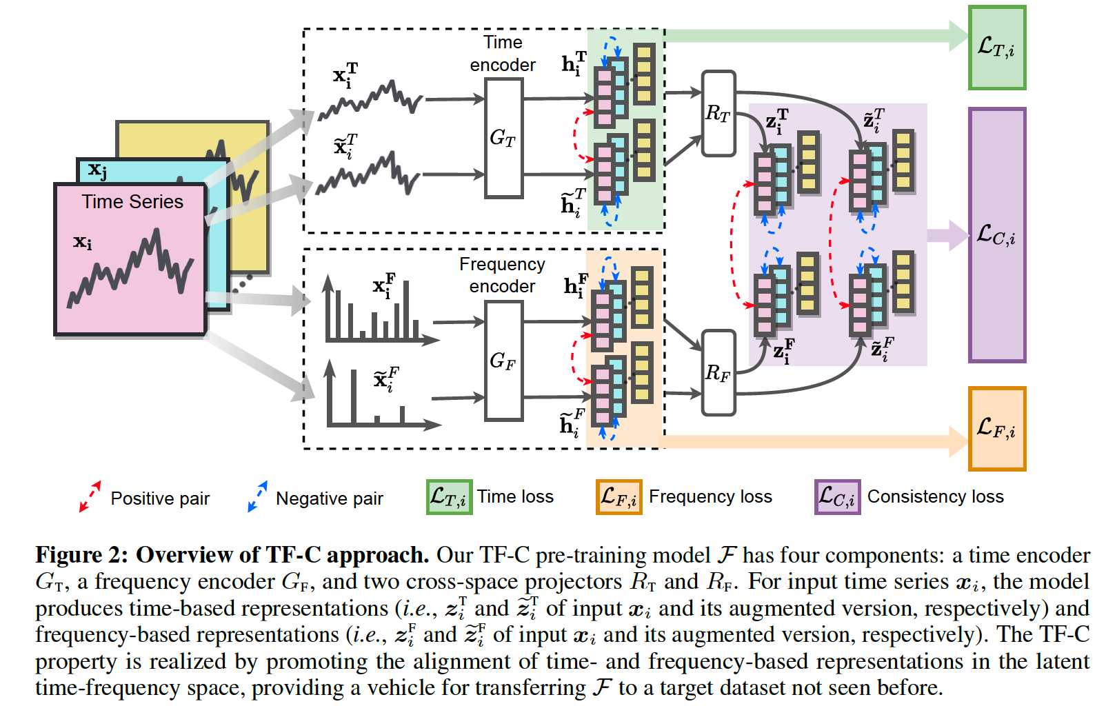
\(\mathcal{F}\) : 4 components

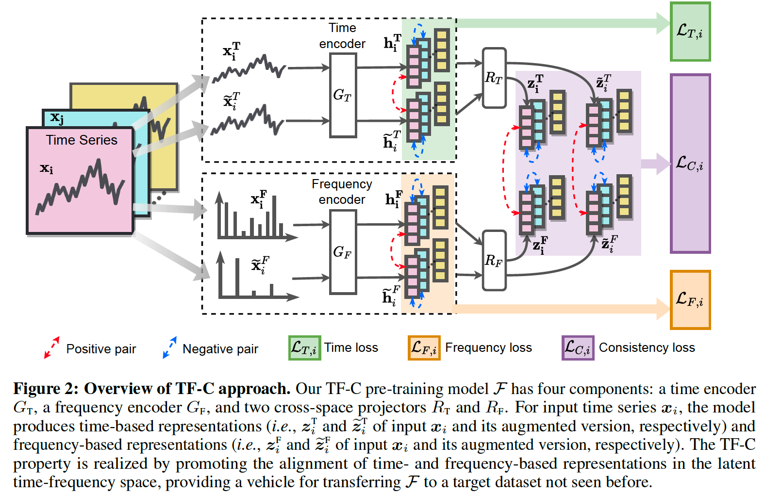
• (1) time encoder : \(G_{\mathrm{T}}\)
• (2) frequency encoder : \(G_{\mathrm{F}}\)
• (3) two cross-space projectors : ( map to time-frequency space )
  • (3-1) for time domain : \(R_{\mathrm{T}}\)
  • (3-2) for frequency domain : \(R_{\mathrm{F}}\)

\(\rightarrow\) 4 components embed \(\boldsymbol{x}_i\) to the latent time-frequency space

Induce (1) & (2) to be close !

• (1) \(\boldsymbol{z}_i^{\mathrm{T}}=R_{\mathrm{T}}\left(G_{\mathrm{T}}\left(\boldsymbol{x}_i^{\mathrm{T}}\right)\right)\)
• (2) \(\boldsymbol{z}_i^{\mathrm{F}}=R_{\mathrm{F}}\left(G_{\mathrm{F}}\left(\boldsymbol{x}_i^{\mathrm{F}}\right)\right)\)

4. Our Approach

(1) Time-based Contrastive Encoder

Data Augmentation

• input : \(\boldsymbol{x}_i\)
• Augmentation : \(\mathcal{B}^{\mathrm{T}}: \boldsymbol{x}_i^{\mathrm{T}} \rightarrow \mathcal{X}_i^{\mathrm{T}}\)
• output : (set) \(\mathcal{X}_i^{\mathrm{T}}\) ……. \(\widetilde{\boldsymbol{x}}_i^{\mathrm{T}} \in \mathcal{X}_i^{\mathrm{T}}\)
  • augmented based on temporal characteristics

Time-based augmentation bank

• ex) jittering, scaling, time-shifts, and neighborhood segments ….
• use diverse augmentations
  • make more robust time-based embeddings!

Procedure

• step 1) randomly select an augmented sample \(\widetilde{\boldsymbol{x}}_i^{\mathrm{T}} \in \mathcal{X}_i^{\mathrm{T}}\)

• step 2) feed into a contrastive time encoder \(G_{\mathrm{T}}\)

  • \(\boldsymbol{h}_i^{\mathrm{T}}=G_{\mathrm{T}}\left(\boldsymbol{x}_i^{\mathrm{T}}\right)\) & \(\widetilde{\boldsymbol{h}}_i^{\mathrm{T}}=G_{\mathrm{T}}\left(\widetilde{\boldsymbol{x}}_i^{\mathrm{T}}\right)\)

  • assume these two are close, if from same \(i\)

    ( far, if different \(i\) )

  • pos & neg pairs :

    • pos pairs : \(\left(\boldsymbol{x}_i^{\mathrm{T}}, \widetilde{\boldsymbol{x}}_i^{\mathrm{T}}\right)\)
    • neg pairs : \(\left(\boldsymbol{x}_i^{\mathrm{T}}, \boldsymbol{x}_j^{\mathrm{T}}\right)\) and \(\left(\boldsymbol{x}_i^{\mathrm{T}}, \widetilde{\boldsymbol{x}}_j^{\mathrm{T}}\right)\)

• step 3) calculate contrastive time loss

Contrastive time loss

• adopt the NT-Xent (the normalized temperature-scaled cross entropy loss)
• \(\mathcal{L}_{\mathrm{T}, i}=d\left(\boldsymbol{h}_i^{\mathrm{T}}, \widetilde{\boldsymbol{h}}_i^{\mathrm{T}}, \mathcal{D}^{\text {pret }}\right)=-\log \frac{\exp \left(\operatorname{sim}\left(\boldsymbol{h}_i^{\mathrm{T}}, \widetilde{\boldsymbol{h}}_i^{\mathrm{T}}\right) / \tau\right)}{\sum_{\boldsymbol{x}_j \in \mathcal{D}^{\text {pret }}} \mathbb{1}_{i \neq j} \exp \left(\operatorname{sim}\left(\boldsymbol{h}_i^{\mathrm{T}}, G_{\mathrm{T}}\left(\boldsymbol{x}_j\right)\right) / \tau\right)}\).
  • where \(\operatorname{sim}(\boldsymbol{u}, \boldsymbol{v})=\boldsymbol{u}^T \boldsymbol{v} /\mid \mid \boldsymbol{u}\mid \mid \mid \mid \boldsymbol{v}\mid \mid\)
  • \(\boldsymbol{x}_j \in \mathcal{D}^{\text {pret }}\) : different TS sample and its augmented sample

(2) Frequency-based Contrastive Encoder

Frequency Transformation

• input : \(\boldsymbol{x}_i\)
• transformation : transform operator \((e . g\)., Fourier Transformation )
• output : \(\boldsymbol{x}_i^{\mathrm{F}}\)

frequency component, denotes a …

• (1) base function (e.g., sinusoidal function for Fourier transformation)

  (2) with the corresponding “frequency and amplitude“

Augmentation

• perturb \(\boldsymbol{x}_i^{\mathrm{F}}\) based on characteristics of frequency spectra
  • perturb the frequency spectrum by adding/removing frequency components
• ( small perturbation in freq spectrum \(\rightarrow\) may cause large change in time domain )

Small Budget \(E\)

use \(E\) in perturbation,

• where \(E\) : # of frequency components we manipulate

To removing frequency components …

\(\rightarrow\) randomly select \(E\) frequency components & set their amplitudes as 0

To add frequency components …

\(\rightarrow\) randomly choose \(E\) frequency components

• from the ones that have smaller amplitude than \(\alpha \cdot A_m\)
• increase their amplitude to \(\alpha \cdot A_m\).
  • \(A_m\) : maximum amplitude
  • \(\alpha\) : pre-defined coefficient ( set \(0.5\) )

Frequency-augmentation bank

• input : \(\boldsymbol{x}_i\)
• augmentation : \(\mathcal{B}^{\mathrm{F}}: \boldsymbol{x}_i^{\mathrm{F}} \rightarrow \mathcal{X}_i^{\mathrm{F}}\)
  • 2 methods : removing or adding
• output : (set) \(\mathcal{X}_i^{\mathrm{F}}\) …….. \(\mid \mathcal{X}_i^{\mathrm{Y}}\mid =2\)

Procedure

• step 1) \(\boldsymbol{h}_i^{\mathrm{F}}=G_{\mathrm{F}}\left(\boldsymbol{x}_i^{\mathrm{F}}\right)\)
• step 2) set pos & neg pairs :
  • pos pairs : \(\left(\boldsymbol{x}_i^{\mathrm{F}}, \tilde{\boldsymbol{x}}_i^{\mathrm{F}}\right)\)
  • neg pairs : \(\left(\boldsymbol{x}_i^{\mathrm{F}}, \boldsymbol{x}_j^{\mathrm{F}}\right)\) and \(\left(\boldsymbol{x}_i^{\mathrm{F}}, \widetilde{\boldsymbol{x}}_j^{\mathrm{F}}\right)\)
• step 3) calculate frequency-based contrastive loss

Contrastive frequency loss

• \(\mathcal{L}_{\mathrm{F}, i}=d\left(\boldsymbol{h}_i^{\mathrm{F}}, \widetilde{\boldsymbol{h}}_i^{\mathrm{F}}, \mathcal{D}^{\text {pret }}\right)=-\log \frac{\exp \left(\operatorname{sim}\left(\boldsymbol{h}_i^{\mathrm{F}}, \widetilde{\boldsymbol{h}}_i^{\mathrm{F}}\right) / \tau\right)}{\sum_{\boldsymbol{x}_j \in \mathcal{D}^{\text {pret }}} \mathbb{1}_{i \neq j} \exp \left(\operatorname{sim}\left(\boldsymbol{h}_i^{\mathrm{F}}, G_{\mathrm{F}}\left(\boldsymbol{x}_j\right)\right) / \tau\right)}\).

(3) Time-Frequency Consistency

Consistency loss \(\mathcal{L}_{\mathrm{C}, i}\)

• to urge the learned embeddings to satisfy TF-C

  \(\rightarrow\) time-based & frequency-based embeddings : CLOSE !

• \(\boldsymbol{z}_i^{\mathrm{T}}=R_{\mathrm{T}}\left(\boldsymbol{h}_i^{\mathrm{T}}\right), \widetilde{\boldsymbol{z}}_i^{\mathrm{T}}=R_{\mathrm{T}}\left(\widetilde{\boldsymbol{h}}_i^{\mathrm{T}}\right)\).
  • map \(\boldsymbol{h}_i^{\mathrm{T}}\) from time space to a joint time-frequency space with \(R_{\mathrm{T}}\)
• \(\boldsymbol{z}_i^{\mathrm{F}}=R_{\mathrm{F}}\left(\boldsymbol{h}_i^{\mathrm{F}}\right), \widetilde{\boldsymbol{z}}_i^{\mathrm{F}}=R_{\mathrm{F}}\left(\widetilde{\boldsymbol{h}}_i^{\mathrm{F}}\right)\).
  • map \(\boldsymbol{h}_i^{\mathrm{F}}\) from frequency space to a joint time-frequency space with \(R_{\mathrm{F}}\)

\(S_i^{\mathrm{TF}}=d\left(\boldsymbol{z}_i^{\mathrm{T}}, \boldsymbol{z}_i^{\mathrm{F}}, \mathcal{D}^{\text {pret }}\right)\),

• distance between \(\boldsymbol{z}_i^{\mathrm{T}}\) and \(\boldsymbol{z}_i^{\mathrm{F}}\)

  ( define \(S_i^{\mathrm{TF}}\), \(S_i^{\widetilde{T}F}\), and \(S_i^{T\widetilde{F}}\) similarly )

don’t consider the distance between \(\boldsymbol{z}_i^{\mathrm{T}}\) and \(\widetilde{\boldsymbol{z}}_i^{\mathrm{T}}\) & distance between \(\boldsymbol{z}_i^{\mathrm{F}}\) and \(\tilde{\boldsymbol{z}}_i^{\mathrm{F}}\)

( where the two embeddings are from the same domain )

• information is already in \(\mathcal{L}_{\mathrm{T}, i}\) and \(\mathcal{L}_{\mathrm{F}, i}\)

intuitively, \(\boldsymbol{z}_i^{\mathrm{T}}\) should be closer to \(\boldsymbol{z}_i^{\mathrm{F}}\) in comparison to \(\tilde{\boldsymbol{z}}_i^{\mathrm{F}}\)

\(\rightarrow\) encourage the proposed model to learn a \(S_i^{\mathrm{TF}}\) < \(S_i^{\mathrm{\tilde{TF}}}\)

\(\rightarrow\) (inspired by the triplet loss) design \(\left(S_i^{\mathrm{TF}}-S_i^{\mathrm{TF}}+\delta\right)\) as a term of consistency loss \(\mathcal{L}_{\mathrm{C}, i}\)

Consistency loss \(\mathcal{L}_{\mathrm{C}, i}\)

\(\mathcal{L}_{\mathrm{C}, i}=\sum_{S_{\text {pair }}}\left(S_i^{\mathrm{TF}}-S_i^{\text {pair }}+\delta\right), \quad S^{\text {pair }} \in\left\{S_i^{\widetilde{\mathrm{T}}\widetilde{\mathrm{F}}}, S_i^{\widetilde{\mathrm{T}}F}, S_i^{T\widetilde{\mathrm{F}}}\right\}\).

• \(S_i^{\text {pair }}\) :
  • time-based embedding (e.g., \(\boldsymbol{z}_i^{\mathrm{T}}\) or \(\left.\widetilde{\boldsymbol{z}}_i^{\mathrm{T}}\right)\)
  • frequency-based embedding ( e.g., \(\boldsymbol{z}_i^{\mathrm{F}}\) or \(\widetilde{\boldsymbol{z}}_i^{\mathrm{F}})\)

(4) Implementation and Technical Details

\(\mathcal{L}_{\text {TF-C }, i}=\lambda\left(\mathcal{L}_{\mathrm{T}, i}+\mathcal{L}_{\mathrm{F}, i}\right)+(1-\lambda) \mathcal{L}_{\mathrm{C}, i}\).

overall loss function : 3 terms

• (1) time-based contrastive loss \(\mathcal{L}_{\mathrm{T}}\)
  • urges the model to learn embeddings invariant to temporal augmentations
• (2) frequency-based contrastive loss \(\mathcal{L}_{\mathrm{F}}\)
  • promotes learning of embeddings invariant to frequency spectrum-based augmentations
• (3) consistency loss \(\mathcal{L}_{\mathrm{C}}\)
  • guides the model to retain the consistency between time-based and frequency-based embeddings.

Implementation

• contrastive losses are calculated within the batch.
• \(\mathcal{F}\) : combination of \(G_{\mathrm{T}}, R_{\mathrm{T}}, G_{\mathrm{F}}\), and \(R_{\mathrm{F}}\).
• final embeddings : \(\boldsymbol{z}_i^{\text {tune }}=\mathcal{F}\left(\boldsymbol{x}_i^{\text {tune }}, \Phi\right)=\left[\boldsymbol{z}_i^{\text {tune, }, \mathrm{T}} ; \boldsymbol{z}_i^{\text {tune, } \mathrm{F}}\right]\)