(paper 59) Large Scale Time-Series Representation Learning via Simultaneous Low and High Frequency Feature Bootstrapping

Large Scale Time-Series Representation Learning via Simultaneous Low and High Frequency Feature Bootstrapping

Contents

1. Abstract
2. Introduction
3. Related Works : SSL for TS
4. Proposed Methods
   1. Domain-guided Augmentations
   2. Low Frequency Features Bootstrapping Module
   3. High ~
   4. Low and High ~

0. Abstract

Most existing Self & Un-supervised TS

• do not capture LOW and HIGH frequency features at the same time

• employ large scale models ( like transformers )
• rely on computationally expensive techniques ( like contrastive learning )

Solution : propose a ..

• (1) non-contrastive self-supervised learning approach
• (2) efficiently captures low and high frequency time varying features

Models

• input : RAW TS
• creates 2 different augmented views ( for 2 branches )
  • 2 branches = online & target network ( like BYOL )
  • allow bootstrapping of the latent representation

BYOL vs Proposed

• (BYOL) backbone encoder is followed by MLP heads

• (Proposed) contains additional “TCN” heads

  \(\rightarrow\) combination of MLP and TCN :

  enables an effective representation of low & high frequency time varying features

  ( due to the varying receptive fields )

1. Introduction

• propose a non-contrastive large scale TS representation learning via simultaneous bootstrapping of low and high frequency input features

• motivated from BYOL

  ( = do not use negative samples … only positive! )

Contributions

• simple yet efficient and novel method
  • which can work without a large pool of labelled data
• noncontrastive self-supervised learning
  • does not require negative pairs
• capture low and high frequency time varying features at the same time.
  • uses MLP and TCN heads
    • capture temporal dependencies at various scales in a complementary manner

2. Related Works : SSL for TS

wide range of pretext tasks have been explored to learn good time-series representation

Pretext-task

• ex) SSL-ECG : predict transformations similar to rotation prediction
• ex) [15] : transformation prediction task for human activity recognition.

Contrastive Learning

• ex) CPC (contrastive predictive coding)

• ex) [16] : extended SimCLR model to EEG data

• ex) [19] : multitask contrastive learning approach
  • capture temporal and contextual information

All existing approaches :

• either rely on “pretext task” or “contrastive learning” or “supervised learning”

  ( \(\rightarrow\) not generalizable and inefficient or need labeled data )

• do not to capture low and high frequency time varying features at the same time

3. Proposed Methods

Procedure

• step 1) generate 2 different augmentations from input TS

• step 2) passed through low frequency and high frequency features bootstrapping module

  • Low frequency feature bootstrapping module :

    • responsible for learning time varying features in low frequency (longer time period)

  • High frequency feature bootstrapping module :

    • responsible for capturing features from short time intervals which contains discontinuities, ruptures and singularities

    \(\rightarrow\) Both modules capture complementary features

(1) Domain-guided Augmentations

choosing correct data augmentations is one of the most important factor

( CV augmentations may not able to work for TS )

Found that creating 2 augmentations from same augmentation family provides better results

• applied jitter-permute-Rotate augmentation
• [Online Network]
  • add random variations to the signal
  • split the signal into a random number of segments with a maximum of \(M\)
  • randomly shuffle them followed by rotation of 30 
• [Target Network]
  • same augmentation ( as target network )
  • but with rotation angle 45

(2) Low Frequency Features Bootstrapping Module

responsible for ….

• (1) capturing low frequency time varying features,

  from the latent representation produced by encoder

  • encoder : large kernel 3 layer CNN ( using TCN )

• (2) bootstrapping learned representation from online network to target network

Procedure

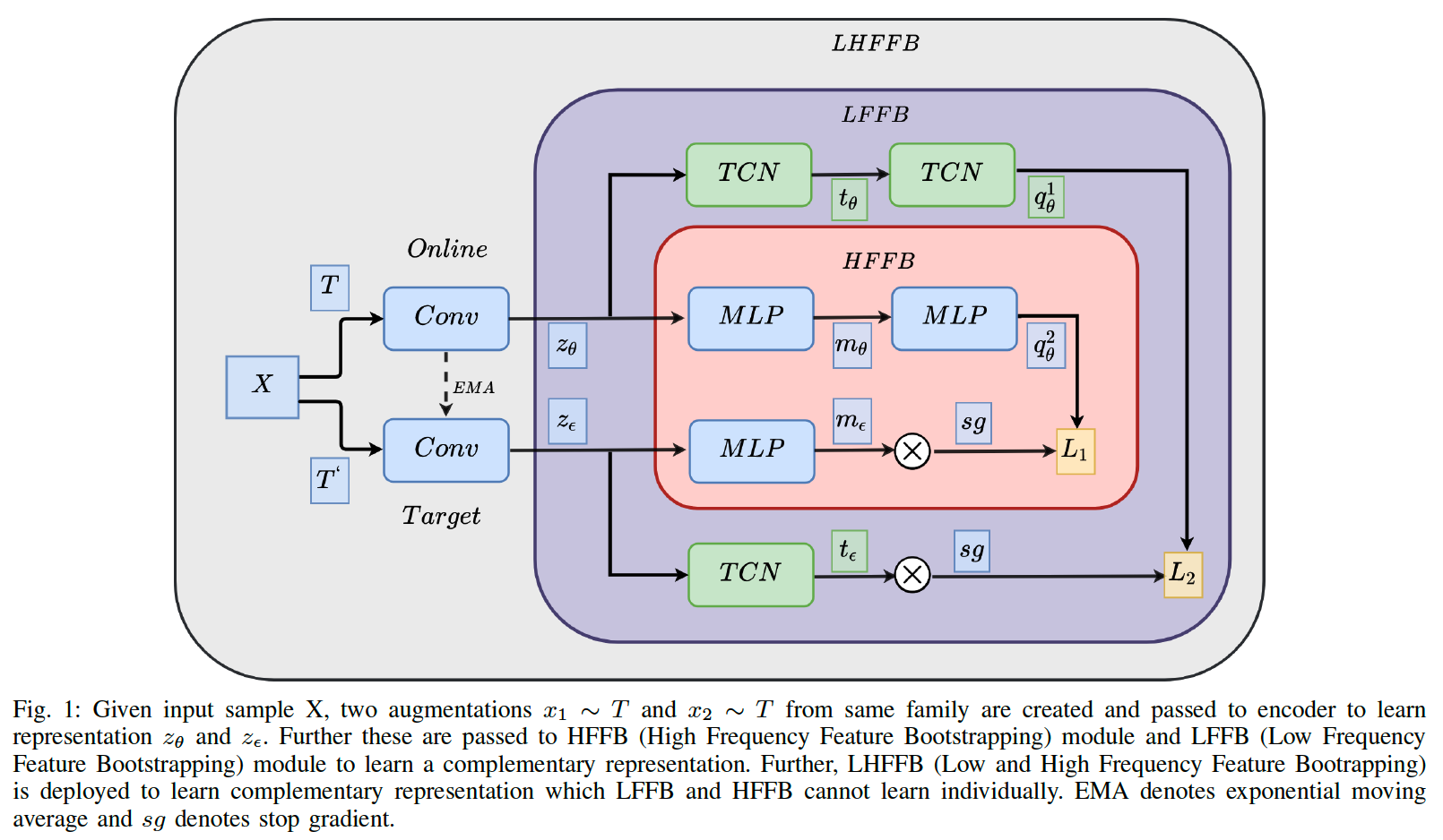
• (1) input : signal \(x\)
• (2) augmentation : \(x_1 \sim T\) and \(x_2 \sim T\)
• (3) encoding : \(z^\theta\) and \(z^\epsilon\)
  • passed through two separate 3-block CNN ( with large kernel size )
  • extract high-dimensional latent representation
    • \(z^\theta=\left[z_1^\theta, z_2^\theta \ldots z_n^\theta\right]\) and \(z^\epsilon=\left[z_1^\epsilon, z_2^\epsilon \ldots z_n^\epsilon\right]\)
  • \(z_i^n=N *\left[\operatorname{Conv}\left(B N \operatorname{Norm}\left(\operatorname{Re} L U\left(\operatorname{Pool}\left(x_i^n\right)\right)\right), K_l\right)\right]\).
    • \(i\) : number of time-stamps
    • \(K_l\) : kernel size
    • \(n\) : parameter ( \(\theta\) for online / \(\epsilon\) for target )
    • \(N\) : number of blocks
  • obtain 2 representations : \(z^\theta\) and \(z^\epsilon\)
• (4) generate low frequency time varying representation \(t_{T C N}^\theta\) and \(t_{T C N}^\epsilon\).
  • with projection heads \(g_{T C N}^\theta\) and \(g_{T C N}^\epsilon\)
  • \(t_i^n=N *\left[\operatorname{TCN}\left(B N \operatorname{orm}\left(\operatorname{Re} L U\left(z_i^n\right)\right), K, D\right)\right]\).
    • \(D\) : dilation rate
• (5) \(t_{T C N}^\theta\) \(\rightarrow\) \(q_{T C N}^\theta\)
  • responsible for predicting representation of \(g_{T C N}^\epsilon\)
• (6) Loss Function : MSE
  • \(\begin{gathered} L_{L F B}= \mid \mid \tilde{q}_{T C N}^\theta-\tilde{g}_{T C N}^\epsilon \mid \mid _2^2 \\ L_{L F B}=2-2 \cdot \frac{\tilde{q}_{T C N}^\theta, \tilde{g}_{T C N}^\epsilon}{ \mid \mid \tilde{q}_{T C N}^\theta \mid \mid \cdot \mid \mid \tilde{g}_{T C N}^\epsilon \mid \mid } \end{gathered}\).

(3) High Frequency Features Bootstrapping Module

Responsible for …

• capturing high frequency representation
• directly bootstrapping representation learned by online network to target network

learn from TS which has shorter time intervals with discontinuities, singularities and ruptures

Procedure ( 1~3 : same as above )

• (1) input : signal \(x\)
• (2) augmentation : \(x_1 \sim T\) and \(x_2 \sim T\)
• (3) encoding : \(z^\theta\) and \(z^\epsilon\)
• (4) generate high frequency time varying representation \(m_{M L P}^\theta\) and \(m_{M L P}^\epsilon\)
  • with projection heads \(g_{M L P}^\theta\) and \(g_{M L P}^\epsilon\)
  • \(m_i^n=N * M L P\left(g_i^n\right)\).
    • \(D\) : dilation rate
• (5) \(m_{M L P}^\theta\) \(\rightarrow\) \(q_{M L P}^\theta\)
  • responsible for predicting representation of \(g_{M L P}^\epsilon\)
• (6) Loss Function : MSE
  • \(\begin{gathered} L_{H F B}= \mid \mid \tilde{q}_{M L P}^\theta-\tilde{g}_{M L P}^\epsilon \mid \mid _2^2 \\ L_{H F B}=2-2 \cdot \frac{\tilde{q}_{M L P}^\theta \cdot \tilde{g}_{M L P}^\epsilon}{ \mid \mid \tilde{q}_{M L P}^\theta \mid \mid \cdot \mid \mid \tilde{g}_{M L P}^\epsilon \mid \mid } \end{gathered}\).

(4) Low and High Frequency Features Bootstrapping Module

• combines both modules to capture complementary features

• responsible for capturing both types of features from data

Loss function

• \(L_{L H F B}=\lambda * L_{L F B}+(1-\lambda) * L_{H F B}\).