(paper 60) Semi-unsupervised Learning for TSC

Semi-unsupervised Learning for TSC

Contents

1. Abstract
2. Introduction
3. Datasets
   1. HAR (Human Activity Recognition)
   2. ECG Heartbeat Classification
   3. Electric Devices
4. Methodology
   1. GMM
   2. GMM for Semi-unsupervised Classification
5. Experiments

0. Abstract

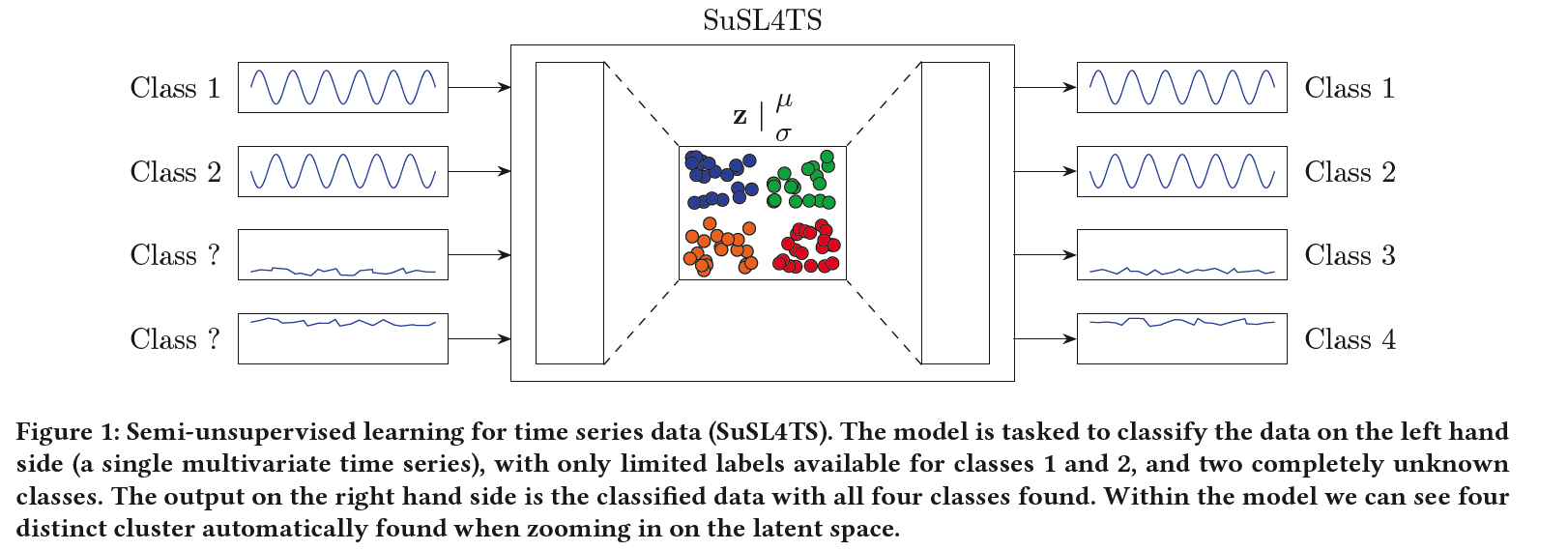
SuSL4TS

• deep generative GMM for semi-unsupervised learning

• classify TS data

• detect sparsely labeled classes (semi-supervised)

  & identify emerging classes hidden in the data (unsupervised).

1. Introduction

(1) VAE

• encode the data distribution in the latent space
• allows training on all variations of data
• can see anomaly detection as a probability rather than a raw score

(2) Classification

• with the development of semi-supervised generative models…able with small amount of data

• problem : need to know all manifestations of classes beforehand.

(3) Clustering

• could cluster the data, needing no label information at all
• problem : lower classification accuracy & need to manually annotate the found clusters

(4) Classification + Clustering : “hybrid approach of semi-unsupervised learning”

\(\rightarrow\) present SuSL4TS

• a convolutional GMM for semi-unsupervised learning on TS data

Contributions

• (1) model capable of semi-unsupervised TSC

• (2) We show the efficacy of our approach on several benchmark datasets

2. Datasets

only hand-select some datasets for our purposes.

3 datasets

• both in the univariate and multivariate setting
• stemming from different domains of data acquisition

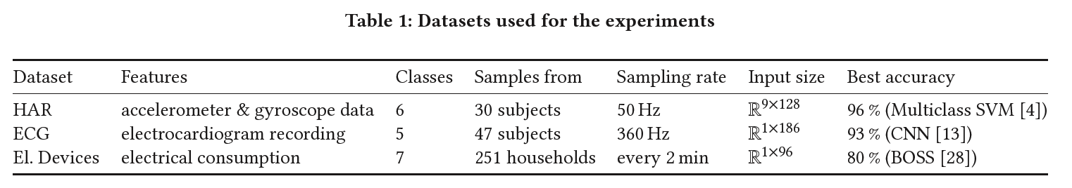
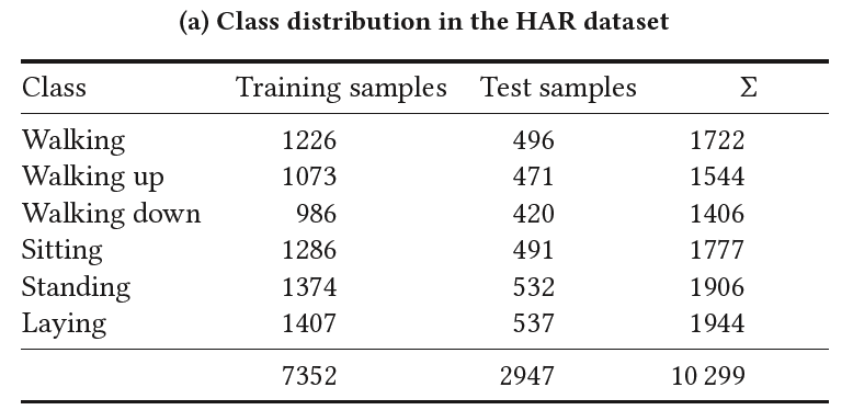
(1) HAR (Human Activity Recognition)

• consists of data collected from accelerometer and gyroscope sensors in smartphones.

• # of subjects = 30

  • tasked with performing various Activities of Daily Living (ADL)

  • instructed to perform six distinct ADL adhering to a defined protocol outlining the order of activities.

    ( standing, sitting, laying down, walking, walking downstairs and walking upstairs )

  • each activity was performed for 15 sec

    • except… walking up and downstairs : 12 sec

  • each activity was performed twice & 5 sec pauses separated activities

• pre-processed for noise reduction

  ( + gravitational and body motion was separated using a low-pass filter )

• 9 signals were sampled with a window of 2.56 sec with 50 % overlap

  ( i.e. input is of size \(R^{9×128}\) )

• A feature vector was obtained from each sampling window

  • 561 features were extracted

• 70/30 training/test split = 7352 / 2947 samples

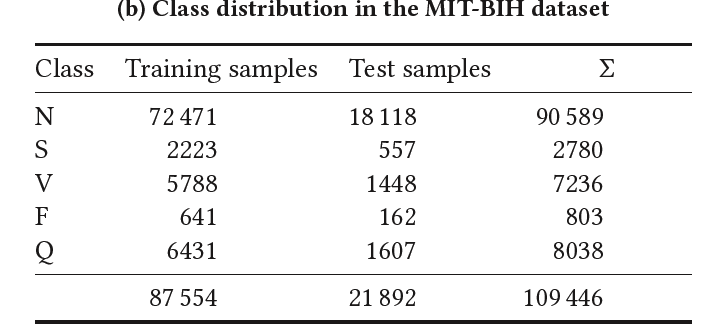
(2) ECG Hearbeat Classification

• consists of electrocardiogram (ECG) recordings

• # of subjects = 47

• grouped in 5 categories

• class frequency is skewed towards the \(N\) class ( = Normal )

• each entry in the set consists of a single heartbeat padded with zeroes

  ( i.e. input is of size \(R^{1×186}\) )

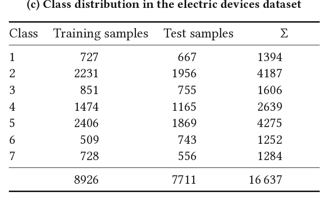
(3) Electric Devices

• Samples are taken every 2 min from 251 households

• After pre-processing and resampling to 15 min averages….

  \(\rightarrow\) length of 96 values ( i.e. input is of size \(R^{1×96}\) )

• regrouping the originally 10 classes to 7

3. Methodology

(1) GMM

• encoder of VAE : \(\Phi(x): \mathbb{R}^n \rightarrow \mathbb{R}^d\)
• decoder of VAE : \(\Theta(z): \mathbb{R}^d \rightarrow \mathbb{R}^n\)
• compressed space is often used for other downstream tasks
• 2 steps
  • step 1) unsupervised
  • step 2) supervised ( downstream )

• 2-step process can be merged into one

  \(\rightarrow\) by adapting the joint probability distribution \(p_{\Theta}\)

  \(\rightarrow\) resulting in a Gaussian Mixture Deep Generative model (GMM)

  ( capable of learning semi-supervised classification )

(2) GMM for Semi-unsupervised Classification

• adapt [7, 30] and replace 2d conv \(\rightarrow\) 1d conv

• use the work shown in [30] in 2 ways
  • 1) use it a reference in performance for the presented convolutional model
  • 2) adapt their idea of **Gaussian \(L_2\) reg )
• overall loss function :
  • \(\begin{aligned} \mathcal{L} &:=\underset{x, y \in D_l}{\mathbb{E}}\left[\mathcal{L}_l(x, y)-\alpha \cdot \log q_{\Phi}(y \mid x)\right] \\ &+\underset{x \in D_u}{\mathbb{E}}\left[\mathcal{L}_u(x)-\gamma \cdot \lambda \cdot \sum_{c \in C} q_{\Phi}(c \mid x) \cdot \log q_{\Phi}(c \mid x)\right] \\ &+w \cdot \Theta_t . \end{aligned}\).

Notation

• \(D_l\) : labeled subset of the data
• \(D_u\) : all unlabeled data
• \(\Theta_t\) : trainable weights at epoch \(t\)
• \(\alpha, \gamma, \lambda\) : hyperparameters weighting the entropy regularization
• loss terms \(\mathcal{L}_l, \mathcal{L}_u\) measure the evidence lower bound (ELBO) from the GMM model

4. Experiments