(paper 61) CA-TCC

Self-supervised Contrastive Representation Learning for Semi-supervised TSC

Contents

1. Abstract
2. Introduction
3. SSL for TS
   1. Pretext Tasks
   2. Contrastive Learning
4. Methods
   1. TS Data Augmentation
   2. Temporal Contrasting
   3. Contextual Contrasting
   4. Class-Aware TS-TCC
5. Experiments

0. Abstract

propose a novel TS representation learning framework

• with TS-TCC ( Temporal and Contextual Contrasting )
• use contrastive learning

propose time-series specific ”weak” and “strong” augmentations

& use their views to

• learn “robust temporal relations” in the proposed temporal contrasting module
• learn “discriminative representations” by our proposed contextual contrasting module

Details

• conduct a systematic study of time-series data augmentation selection

• extend TS-TCC to the semi-supervised learning sestings

  \(\rightarrow\) propose a Class-Aware TS-TCC (CA-TCC)

  • benefits from the available few labeled data
  • leverage robust pseudo labels produced by TS-TCC to realize class-aware contrastive loss.

1. Introduction

Contrastive learning

• strong ability over pretext tasks
• ability to learn invariant representations by contrasting different views of the input sample ( via augmentation )

image-based contrastive learning methods

• may not able to work on TS

Why?

• reason 1) where its features are mostly spatial, we find time-series data are mainly characterised by the temporal dependencies
• reason 2) augmentation techniques used for images such as color distortion, generally cannot fit well with TS data

Proposal

• propose a novel framework, that incorporates contrastive learning into self- and semi-supervised learning
• propose a Time-Series representation learning framework via Temporal and Contextual Contrasting (TS-TCC), that is trained on totally unlabeled datasets
  • employs 2 contrastive learning & augmentation techniques
• propose simple yet efficient data augmentations
  • that can fit any TS to create 2 different, but correlated views of the input samples
  • then used by the 2 innovative contrastive learning modules
• (module 1) temporal contrasting module
  • learn robust representations by designing a tough cross-view prediction task
• (module 2) contextual contrasting module
  • learn discriminative representations
  • aim to maximize the similarity among different contexts of the same sample while minimizing similarity among contexts of different samples

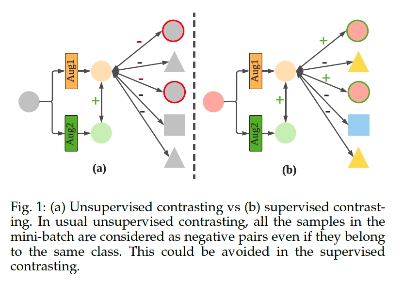
Limitation of the contextual contrasting :

• contrasting samples from the same class will be treated as negative pairs

  ( since label information is not available )

• propose another variant for Class-Aware TS-TCC (CA-TCC) to utilize class information when contrasting between samples

2. SSL for TS

(1) Pretext Tasks

• ex) [25] binary classification pretext task for HAR
  • by applying several transformations
  • classify between the original &transformed
• ex) [26] SSL-ECG
  • ECG representations are learned by applying 6 transformations
  • assigned pseudo labels according to the transformation type
  • classify these transformations
• ex) [27] designed 8 auxiliary tasks
• ex) [28] subject-invariant representations by modeling local and global activity patterns

(2) Contrastive Learning

• ex) CPC ( Contrastive Predictive Coding )

  • by predicting the future in the latent space
  • great advances in various speech recognition

• ex) [29] : studied 3 self-supervised tasks with 2 pretext tasks & 1 contrastive task

  • pretext 1) relative positioning
  • pretext 2) temporal shuffling
  • contrastive 1) uses CPC to learn representations about clinical EEG data

  \(\rightarrow\) representations learned by CPC perform the best

  \(\rightarrow\) CL generally perform better than the pretext tasks

• ex) [9] : designed EEG related augmentations & extended SimCLR

Existing approaches : use either TEMPORAL or GLOBAL features

\(\leftrightarrow\) proposed : address both types of features

• in our (1) cross-view temporal and (2) contextual contrasting modules.

3. Methods

Preliminaries : TS-TCC

Starting with TS-TCC

• step 1) generate 2 different yet correlated views of the input data

  • based on strong and weak augmentations

• step 2) temporal contrasting module

  • explore the temporal features of the data with 2 autoregressive models

  • perform a tough cross-view prediction task,

    by predicting the future of one view using the past of the other

• step 3) contextual contrasting module

  • maximize the agreement between the contexts of the AR models

(1) TS Data Augmentation

Data augmentation

• key part in the success of the contrastive learning

• Usually, contrastive learning methods use 2 (random) variants of the same augmentation

However, we argue that producing views from DIFFERENT augmentations can improve the robustness of the learned representations

\(\rightarrow\) propose 2 separate augmentations

• ver 1) weak
• ver 2) strong

Strong & Weak augmentation

strong augmentation

• to enable the tough cross-view prediction task in the next module
• helps in learning robust representations

weak augmentation

• aims to add some small variations to the signal without affecting its characteristics

Notation

• input : \(x\)
• strong & weak sample : \(x^s \sim \mathcal{T}_s\) and \(x^w \sim \mathcal{T}_w\)
  • then passed to the encoder
• Encoder : \(\mathbf{z}=f_{e n c}(\mathbf{x})\)
  • 3 block convolutional architecture
• Encoded : \(\mathbf{z}=\left[z_1, z_2, \ldots z_T\right]\)
  • where \(T\) is the total timesteps, \(z_i \in \mathbb{R}^d\), where \(d\) is the feature length
• Encoded ( weak & strong ) : \(\mathbf{z}^s\) & \(\mathbf{z}^w\)
  • then fed into the temporal contrasting module

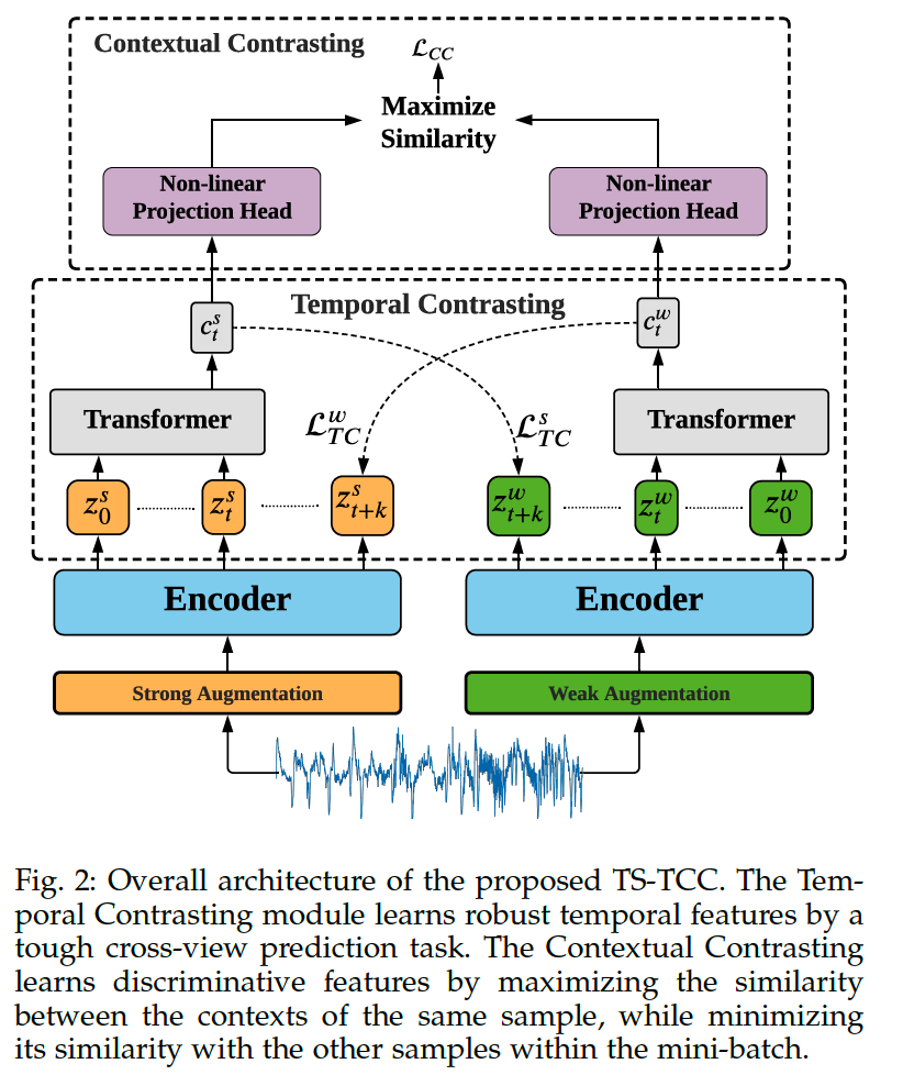
(2) Temporal Contrasting

• deploys a contrastive loss to extract temporal features
• with an AR model ( \(f_{\text {ar }}\) )
  • generates context vector : \(c_t=f_{a r}\left(\mathbf{z}_{\leq t}\right), c_t \in \mathbb{R}^h\)
    • \(h\) is the hidden dimension of \(f_{a r}\)
  • \(c_t\) is then used to predict the timesteps from \(z_{t+1}\) until \(z_{t+k}(1<k \leq K)\)
    • use log-bilinear model … \(f_k\left(x_{t+k}, c_t\right)=\exp \left(\left(\mathcal{W}_k\left(c_t\right)\right)^T z_{t+k}\right)\)
• strong & weak
  • strong augmentation : generates \(c_t^s\)
  • weak augmentation : generates \(c_t^w\)
• propose a tough cross-view prediction task
  • use \(c_t^s\) to predict future timesteps of \(z_{t+k}^w\)
  • use \(c_t^w\) to predict future timesteps of \(z_{t+k}^s\)

• contrastive loss :

  \( \begin{gathered} \mathcal{L}_{T C}^s=-\frac{1}{K} \sum_{k=1}^K \log \frac{\exp \left(\left(\mathcal{W}_k\left(c_t^s\right)\right)^T z_{t+k}^w\right)}{\sum_{n \in \mathcal{N}_{t, k}} \exp \left(\left(\mathcal{W}_k\left(c_t^s\right)\right)^T z_n^w\right)} \\ \mathcal{L}_{T C}^w=-\frac{1}{K} \sum_{k=1}^K \log \frac{\exp\left(\left(\mathcal{W}_k\left(c_t^w\right)\right)^T z_{t+k}^s\right)}{\sum_{n \in \mathcal{N}_{t, k}} \exp \left(\left(\mathcal{W}_k\left(c_t^w\right)\right)^T z_n^s\right)}\end{gathered}\).

  
  

Transformer

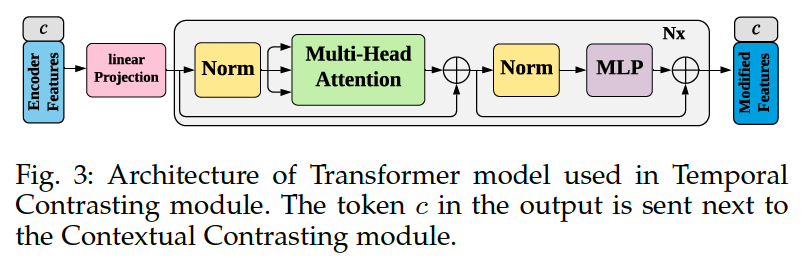
• use Transformer as the AR model
• mainly consists of multi-headed attention (MHA) followed by a Multilayer Perceptron (MLP)
  • MLP : 2 FC layer + ReLU + dropout
• use Pre-norm residual connections
• stack \(L\) identical layers to generate the final features
• add a token \(c \in \mathbb{R}^h\) to the input
  • acts as a representative context vector in the output

Procedures

• step 1) linear projection
  • apply \(\mathbf{z}_{\leq t}\) to a linear projection \(\mathcal{W}_{\text {Tran }}: \mathbb{R}^{d \rightarrow h}\)
  • maps the features into the hidden dimension
• step 2) sent to the Transformer
  • \(\tilde{\mathbf{z}}=\mathcal{W}_{\operatorname{Tran}}(\mathbf{z}_{\leq t}), \quad \tilde{\mathbf{z}} \in \mathbb{R}^h\).
• step 3) attach the context vector into the feature vector \(\tilde{\mathbf{z}}\)
  • input features become \(\psi_0=[c ; \tilde{\mathbf{z}}]\)
• step 4) pass \(\psi_0\) through Transformer layers
  • \(\tilde{\psi}_l =\operatorname{MHA}\left(\operatorname{Norm}\left(\psi_{l-1}\right)\right)+\psi_{l-1}, 1 \leq l \leq L\).
  • \(\psi_l =\operatorname{MLP}\left(\operatorname{Norm}\left(\tilde{\psi}_l\right)\right)+\tilde{\psi}_l,1 \leq l \leq L\).
• step 5) re-attach the context vector from the final output
  • \(c_t=\psi_L^0\) ….. be the input of the contextual contrasting module

(3) Contextual Contrasting

aims to learn more discriminative representations

Procedures

• step 1) apply a non-linear transformation to the contexts

  • via projection head

    • maps the contexts into the space where the contextual contrasting is applied

  • ex) given a batch of N input samples … will have 2 contexts for each sample

    \(\rightarrow\) Have \(2N\) contexts

  • Notation ) for context \(c_t^i\) ….

    • positive sample : \(c_t^{i^{+}}\)
    • positive pair : \(\left(c_t^i, c_t^{i^{+}}\right)\)
    • negative samples : remaining \((2 N-2)\) contexts

• step 2) Contextual Contrasting Loss ( \(\mathcal{L}_{C C}\) )

  • \(\begin{aligned} &\ell\left(i, i^{+}\right)=-\log \frac{\exp\left(\operatorname{sim}\left(c_t^i, c_t^{i+}\right) / \tau\right)}{\sum_{m=1}^{2 N} \mathbb{1}_{[m \neq i]} \exp \left(\operatorname{sim}\left(c_t^i, c_t^m\right) / \tau\right)} \\&\mathcal{L}_{C C}=\frac{1}{2 N} \sum_{k=1}^{2 N}[\ell(2 k-1,2 k)+\ell(2 k, 2 k-1)]\end{aligned}\).
    • \(\operatorname{sim}(\boldsymbol{u}, \boldsymbol{v})=\boldsymbol{u}^T \boldsymbol{v} / \mid \mid \boldsymbol{u} \mid \mid \mid \mid \boldsymbol{v} \mid \mid\).

• step 3) Overall SSL Loss :

  • (1) temporal contrasting loss
  • (2) contextual contrasting loss

  \(\rightarrow\) \(\mathcal{L}_{\text {unsup }}=\lambda_1 \cdot\left(\mathcal{L}_{T C}^s+\mathcal{L}_{T C}^w\right)+\lambda_2 \cdot \mathcal{L}_{C C}\)

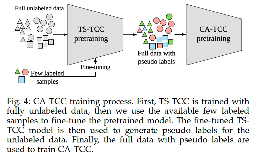
(4) Class-Aware TS-TCC

second variant of our framework :

• use of few labeled data

  ( to further improve the representation learned by TS-TCC )

• aim to overcome one drawback in the contextual contrasting module : considering all the samples in mini-batch as negative pairs

• solution : CA TCC

CA TCC ( Class-Aware TS-TCC )

• replace the contextual contrasting with a ”supervised” contextual contrasting

Supervised contrastive learning

• first proposed to improve the supervised CE loss
• reuse it in our framework to improve the contextual contrasting
• instead of having a single positive pair (from augmented views), we use multiple instances from the same class as positive pairs

BUT … requires the availability of the “full” labeled data

\(\rightarrow\) in CATCC, make use of the available “few” labeled samples to fine-tune the pretrained TS-TCC.

• then, fine-tuned model is used to generate pseudo labels for the unlabeled data

  & use these pseudo labels to train our CA-TCC

Notation

• \(N\) labeled samples \(\left\{\mathbf{x}_k, y_k\right\}_{k=1 \ldots N}\)
• after augmentations) \(2 N\) samples, \(\left\{\hat{\mathbf{x}}_l, \hat{y}_l\right\}_{l=1 \ldots 2 N}\)
  • such that \(\hat{\mathbf{x}}_{2 k}\) and \(\hat{\mathbf{x}}_{2 k-1}\) are the two views of \(\mathbf{x}_k\)
  • \(y_k=\hat{y}_{2 k}=\hat{y}_{2 k-1}\).
• \(A(i) \equiv I \backslash\{i\}\),
• supervised contextual contrasting loss
  • \(\mathcal{L}_{S C C}=\sum_{i \in I} \frac{1}{ \mid P(i) \mid } \sum_{p \in P(i)} \ell(i, p)\).
    • \(P(i)=\left\{p \in A(i): \hat{y}_p=\hat{y}_i\right\}\) : indices of all samples with same class as \(\hat{\mathbf{x}}_i\) in a batch
    • \(\mid P(i) \mid\) : cardinality of \(P(i)\)

  
  

Overall Loss :

• \(\mathcal{L}_{\text {semi }}=\lambda_3 \cdot\left(\mathcal{L}_{T C}^s+\mathcal{L}_{T C}^w\right)+\lambda_4 \cdot \mathcal{L}_{S C C}\).

4. Experiments

Evaluate on 3 different training settings

• (1) linear evaluation
• (2) semi-supervised training
• (3) transfer learning

2 metrics

• (1) accuracy
• (2) macro-averaged F1-score (MF1)
  • for imbalanced datasets

(1) Comparison with Baselines

Baselines

• (1) Random Initialization:
  • training a linear classifier on top of frozen and randomly initialized encoder
• (2) Supervised:
  • supervised training of both encoder and classifier
• (3) SSL-ECG
• (4) CPC
• (5) SimCLR
  • use our timeseries specific augmentations to pretrain SimCLR
• (6) FixMatch
  • relies on weak and strong augmentations in training
  • trained it using our proposed augmentations

To evaluate the performance of SSL-ECG, CPC, SimCLR and TS-TCC ….

• step 1) pretrain ( w.o labeled data )
• step 2) evaluation ( with a portion of the labeled data )
  • standard linear evaluation scheme
  • train a linear classifier on top of a frozen SSL pretrained encoder model

Accuracy ( with LIMITED labeled dataset )

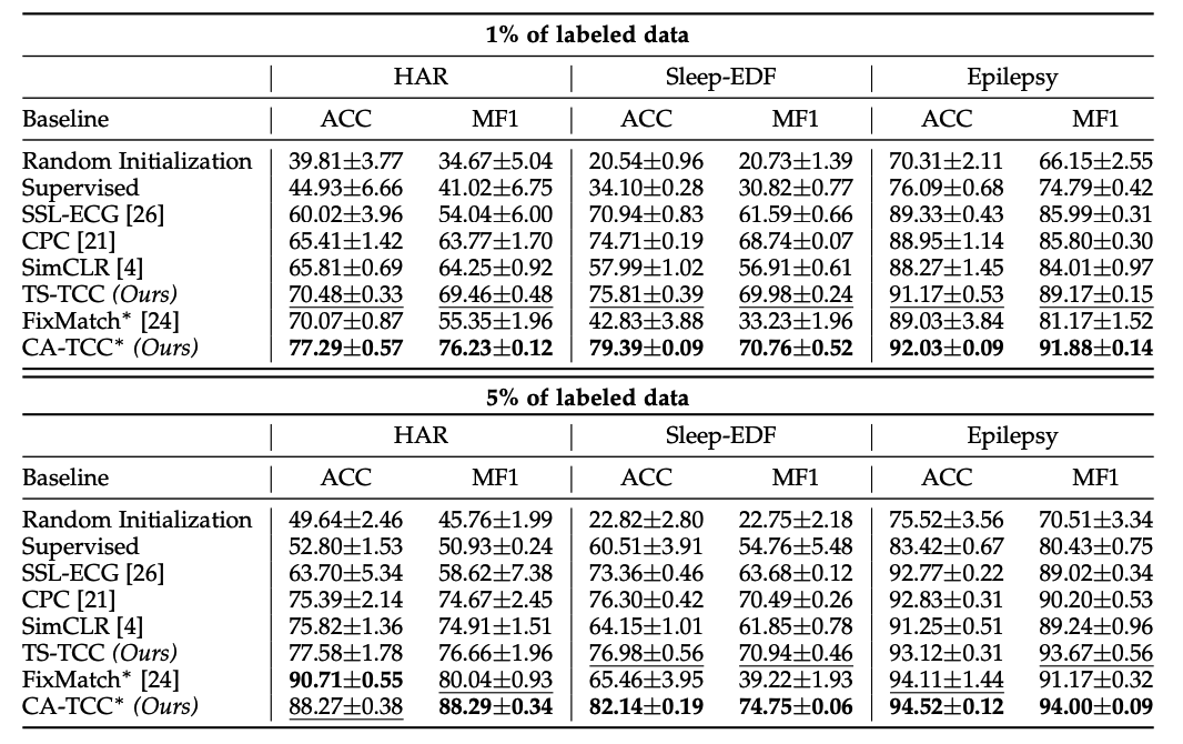
Implications

• contrastive methods > pretext-based method
  • contrastive methods : CPC, SimCLR and our TS-TCC
  • pretext-based method : SSL-ECG
• CPC > SimCLR
  • temporal features are more important than general features in TS data

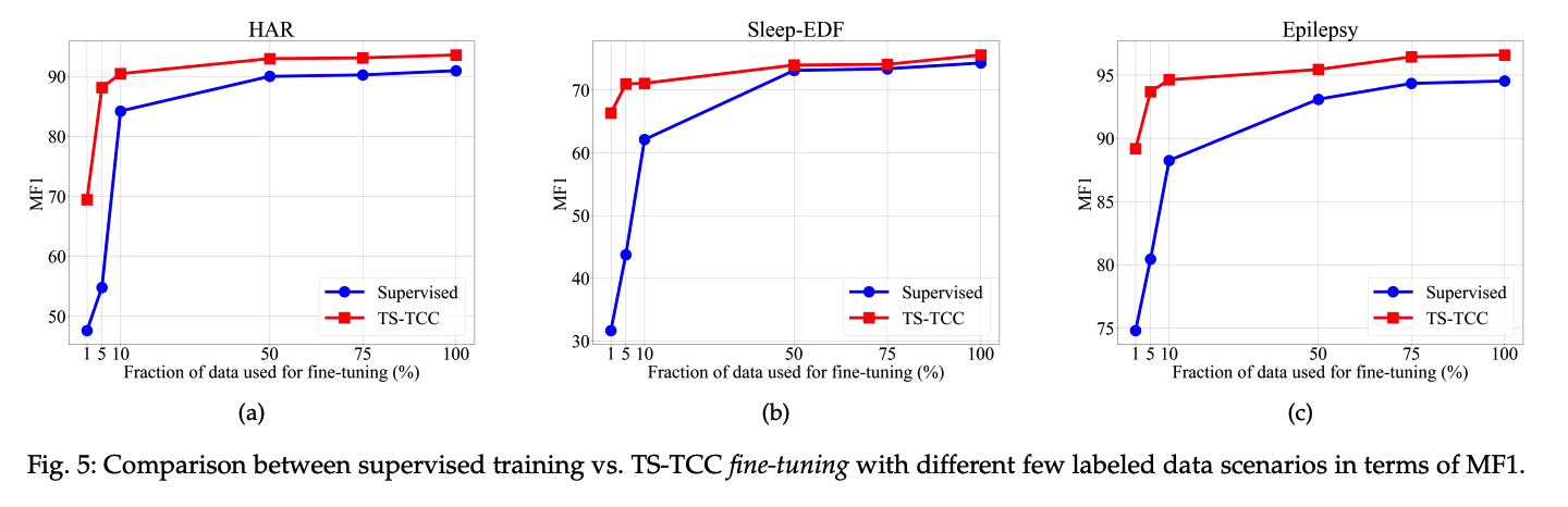
(2) Semi-supervised Experiments

investigate TS-TCC, under different semi-supervised settings

• fine-tune the pretrained model using 1%, 5%, 10%, 50%, 75% data
• metric : MF1 ( \(\because\) imbalance of Sleep-EDF )

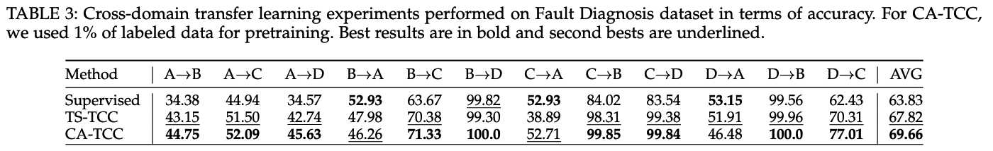
(3) Transfer Learning

Dataset : Fault Diagnosis (FD)

• has 4 working conditions ( = 4 domains, A/B/C/D )

Process

• step 1) train the model on the data from one condition (i.e., source domain)
• step 2) test it on another condition (i.e., target domain)

3 training schemes on the source domain

• (1) Supervised training
• (2) TS-TCC fine-tuning
• (3) CATCC fine-tuning

(2) TS-TCC fine-tuning & (3) CA-TCC fine-tuning

• fine-tune our pretrained encoder using the labeled data in the source domain