(paper 62) SSL for TS Anomaly Detection

SSL for TS Anomaly Detection in Industrial Internet of Things

Contents

1. Abstract
2. Introduction
   1. 2 types of abnormality
   2. TS AD
   3. AD methods
   4. Proposal
3. Related Works
   1. Traditional AD
   2. SSL for AD
4. Data Preprocessing
   1. Data Collection & Preprocessing
   2. Sliding Sample
5. Methodology
   1. SSL
   2. AD

0. Abstract

proposes an AD methodm using a SSL framework in TS darta

TS data augmentation for generating pseudo-label

Classifier : 1d-CNN

• will measure the degree of abnormality

1. Introduction

(1) 2 types of abnormality

• (1) point anomaly : single data point
• (2) collective anomaly : continuous sequence of data points considered anomalous as a whole

(2) TS anomaly detection

• aims to isolate anomalous subsequences of varying lengths

• simple technique : Thresholding

  • detects data points that are outside their range of normal

  ( Unfortunately, many anomalies do not cross any boundaries; for example, contextual anomalies : may have “normal” values but are unusual at the time they occur )

  \(\rightarrow\) difficult to detect

(3) Anomaly detection methods

a) various statistical methods

ex) Statistical Process Control

• detected as an anomaly if it fails to pass statistical hypothesis testing
• huge amount of human knowledge is still necessary to set prior assumptions for the models

b) unsupervised ML approach

ex) segmenting a TS into subsequences of a certain length

& applying clustering algorithms

ex) deep anomaly detection (DAD)

learn hierarchical discriminative features from historical TS

either predicts or reconstructs a TS

( high prediction or reconstruction errors = anomalies )

• cons)

  • inflexible enough in traditional approaches

  • edge devices lack dynamic and automatically updated detection models for various contexts
  • difficult to obtain a large amount of anomalous data

(4) Proposal

novel solution for automatic TS AD on edge device

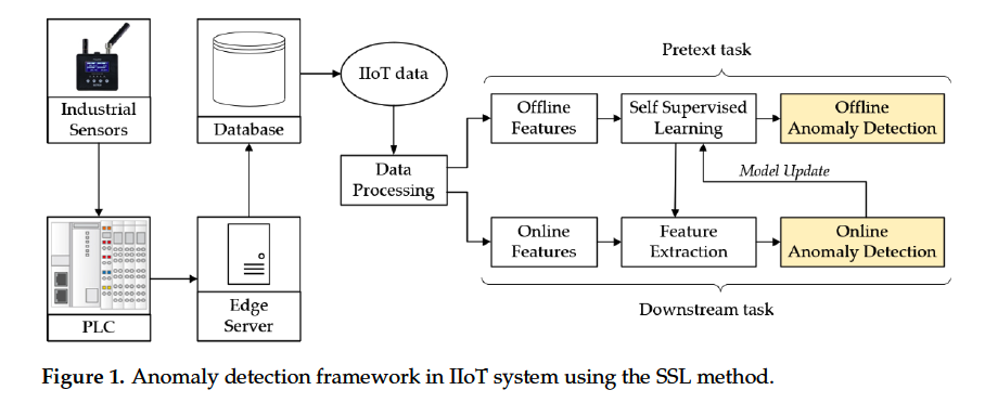
introduces an efficient realtime framework with 2 phases

• (1) offline training
• (2) online inference

a) offline training

• selects historical data from the DB for model training

• DL is provided for automatically detecting the anomalies, using SSL

• only the normal data is learned in the training process

  \(\rightarrow\) explore the features of the supposedly “normal” TS

b) online inference

• employed in real time
• model is updated if the number of abnormal samples is greater than a specified threshold

2. Related Works

(1) Traditional AD

[training] only normal data is provided

[testing] model predicts whether a test sample is normal

various algorithms based on DAD : divided into 3 categories

• (1) Supervised DAD

  • uses the labels of normal and abnormal data
  • ex) [2] employed LR + RF for AD and their categorization
  • ex) [3] based on LSTM with statistical properties

• (2) Semi-supervised DAD

  • ex) [4] employed DBN (Deep Belief Nets)
  • ex) [12] proposed 2 semi-supervised models, based on the generative feature of VAE
  • still requires that the relationship between labeled & unlabeled data distn holds during data collection

• (3) Unsupervised DAD

  • trained using the normal data

    \(\rightarrow\) when data falls outside some boundary condition, considered anomaly

  • VAE, GANs are trained to generate normal data

  • either (1) predict or (2) reconstruct TS

  • ex) [20] : One-class GAN (OCGAN) to improve robustness using a denoising AE

  • ex) [15] : LSTM–Gauss–NBayes

    • stacked LSTM : forecast the tendency of the TS
    • NBayes : detect anomalies based on the prediction result

(2) SSL for AD

SSL process : separated into 2 successive tasks

• (1) pretext task training
• (2) downstream task training

Inspired by the SSL approach for AD…

\(\rightarrow\) propse new solution! based on augmentation of TS

( first to apply principles of the SSL to TS for AD )

• transform TS to different sequences, using the rotation and jittering method before training a classifier ( = trained based on normal data )
• inconsistency when training with abnormal data could be used as

3. Data Preprocessing

(1) Data Collection & Preprocessing

Historical TS is extracted from the DB for data preprocessing

Data preprocessing :

• raw data \(\mathbf{X}=\left(x^1, x^2, x^3, \ldots, x^S\right)\),
  • where \(x^i \in \mathbb{R}^{M \times 1}\) indicates \(\mathrm{M}\) feature at sample \(i\)
  • \(S\) : total sample of the raw data collection

Process

• step 1) Convert timestamps into the same interval
  • inconsistency of the timestamps may occur
• Step 2) Clean data
  • data collection may obtain some missing value due to the different types and impacts
  • alignment of data timestamps also causes missing values
  • ex) k-nearest neighbor imputation
• Step 3) Integrate multiple-sensor feature into single MTS
• Step 4) Scale MTS
  • for sustainable learning process
  • use StandardScaler : \(x_{m(\text { scaler })}^i=\frac{x_m^i-\mu(x)}{\sigma(x)}\)
    • \(x_{m \text { (scaler) }}^i\) : scaled value for the \(m\) th feature
    • \(x_m^i\), the \(m\) th feature from time

(2) Sliding Sample

appy the sliding window to generate TS data containing the time dependence

• \[\mathbf{X}_{T S}=\left\{x_{s e q}^{(n)}\right\}_{n=1}^N\]

Each data has \(T\) steps

• \(x_{\text {seq }}^{(n)}=\left(x_1^{(n)}, x_2^{(n)}, x_3^{(n)}, \ldots, x_T^{(n)}\right)\).
  • \(x^t \in \mathbb{R}^{N \times T}\) : \(\mathrm{N}\) dim of measurements at time step \(t\)

Goal of TS-AD :

• find a set of anomalous time sequences \(\mathbf{A}_{\mathrm{seq}}=\left(a_{\mathrm{seq}}^1, a_{\mathrm{seq}}^2, a_{\mathrm{seq}}^3, \ldots, a_{\mathrm{seq}}^k\right)\),
  • \(a_{\text {seq }}^i\) : continuous sequence of data points in time that show anomalous values within the segment

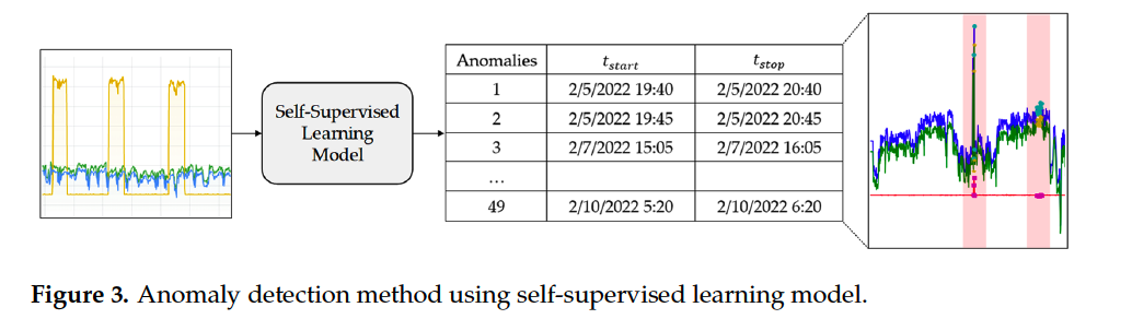
• size of the sequence window (timestep) : \(T = 300\)

4. Methodology

divided into 2 phases

• (1) offline training

  • SSL pretext task training

  • contains historical TS data

  • step 1) TS is first fed into preprocessing scheme

  • step 2) deploy DA based on jittering./rotation for pseudo-label

  • step 3) feature of each TS is fed into classifier

    • determine which scaling transformation should be employed

  • trained on normal TS data

    \(\rightarrow\) maximize the loss, when identifying an anomlay sequence

• (2) online monitoring

  • use what we learned in the offline phase, for downstream tasks

(1) SSL

Goal : learn useful representations of the input data w.o annotation

employ a new architecture for the TS

• pseudo label was generated based on the jittering and rotation
• identification model for predicting the scaled transformation

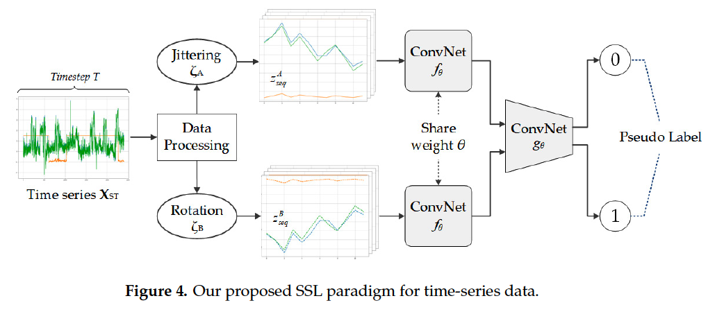
Jittering :

• presupposes that noisy TS are common
• \(\zeta_A\left(x_{\text {seq }}^{(n)}\right)=x_1^{(n)}+\varepsilon_1, x_2^{(n)}+\varepsilon_2, \ldots, x_T^{(n)}+\varepsilon_T,\).
  • \(\varepsilon \sim \mathbb{N}\left(0, \sigma^2\right)\).
    • \(\sigma\) : pre-determined hyperparameter
• Adding noise to the inputs is a well-known method for increasing the generalization

Rotation :

• can change the class associated with the original sample
• \(\zeta_B\left(x_{\text {seq }}^{(n)}\right)=R\left(x_1^{(n)}\right), R\left(x_2^{(n)}\right), \ldots, R\left(x_T^{(n)}\right)\).
  • \(R\left(x_t^{(n)}\right)=-x_t^{(n)}\).
  • \(R\) : element-wise rotation matrix that flips the sign of the original TS

Summary :

• added with noise and flipped by \(\zeta_A\) and \(\zeta_B\).

• TS matrix : \(\mathbf{X}_{T S}\)

• each sequence of data \(x_{\text {seq }}\) : transformed into new sequences…

  • \(\mathbf{z}_{\text {seq }}^A\) : by jittering equation \(\zeta_A\left(x_{s e q}\right)\)
  • \(\mathbf{z}_{\text {seq }}^B\) : by rotation equation \(\zeta_B\left(x_{s e q}\right)\)

• new sequences were finally gathered

  \(\rightarrow\) form \(\mathbf{Z}_{s e q}^A\) and \(\mathbf{Z}_{\mathrm{seq}}^B\)

Final output :

• consisted of two different values
• each representing the probability of jittering data & rotation data

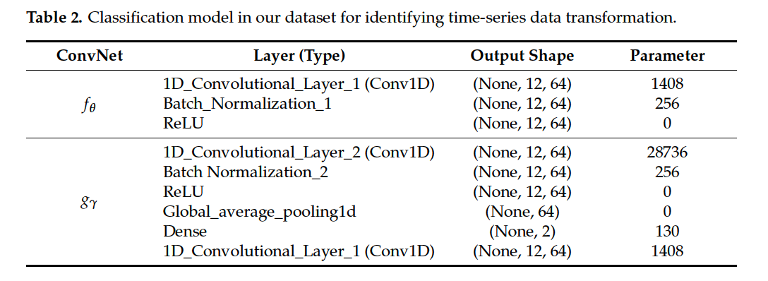
(2) AD

Once \(g_\gamma\) was trained ( based on the self-labeled )

• (Normal) expected to be correctly identified by classifier
• (Abnormal) likely mislead the classifier into predicting the probability of jittering and rotated data

Discrepancy between the

• (1) predicted output by the classifier output
• (2) ground truth of input data

\(\rightarrow\) indicate the degree of abnormality

New data \(x_{\text {seq }}^{(i)}\), DA technique \(\zeta\) was applied to generate a new dataset \(\zeta\left(\mathbf{X}_{T S}\right)\) with pseudo label

Degree of the anomality :

• \(\mathcal{L}\left(f_\theta\left(\zeta\left(\mathbf{X}_{T S}\right)\right), y\right)=-\frac{1}{N} \sum_{i=1}^N\left[y_i \log \left(\hat{y}_i\right)+\left(1-\hat{y}_i\right) \log \left(1-\hat{y}_i\right)\right]\).
• set the threshold for AD, based on the max values of the CE loss function in the training dataset