(paper 64) Mixing Up CL ; SSL for TS

Mixing Up Contrastive Learning: Self-Supervised Representation Learning for Time Series

Contents

1. Abstract
2. Introduction
3. Method
   1. Training on labeled data
   2. Training on unlabeled data
4. Experiments

0. Abstract

propose an unsupervised CL

• motivated from the perspective of label smoothing

• uses a novel contrastive loss,

  that naturally exploits a data augmentation scheme

  in which new samples are generated by mixing two data samples

• task : predict the mixing component

  • utilized as soft targets in the loss function

1. Introduction

introduces a novel SSL, that exploits “mixup”

mixup data augmentation

• creates an augmented sample,

• through a convex combination of 2 data points

  \(\rightarrow\) allows for generation of new data points ( = augmented samples )

Task :

• predict the strength of the mixing component

• based on the “2 data points” and the “augmented sample”

( motivated by label smoothing )

Label Smoothing

• has been shown to increase performance & reduce overconfidence

Datasets :

• UCR (Dau et al., 2018)
• UEA (Bagnall et al., 2018)

2. Mixup Contrastive Learning

CL for TS

• propose a new contrastive loss,

  that exploits the information from the data augmentation procedure.

Notation

• ( also applicable to MTS, but introduce with UTS )

• UTS : \(x=\{x(t) \in \mathbb{R} \mid t=1,2, \cdots, T\}\)

  ( vectorial data : \(\mathbf{x}\) )

Data Augmentation ( for TS )

• potential invariances of TS are rarely known in advance

• In this work ….

  \(\rightarrow\) data augmentation based on mixup

Mixup

• 2 time series \(x_i\) and \(x_j\) drawn randomly
• augmented training example : \(\tilde{x}=\lambda x_i+(1-\lambda) x_j\)
  • \(\lambda \in[0,1]\) …. \(\lambda \sim \operatorname{Beta}(\alpha, \alpha)\) and \(\alpha \in(0, \infty)\)

(1) A Novel Contrastive Loss for Unsupervised Representation Learning of TS

Procedure

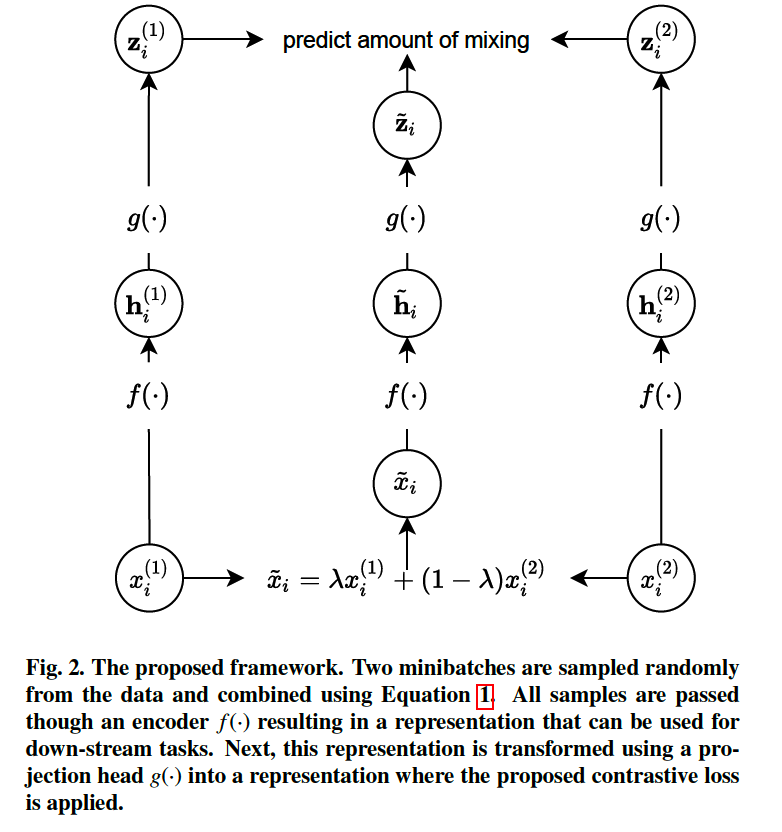
At each training iteration…

• \(\lambda\) is drawn randomly ( from a beta distn )

• 2 mini- batches of size \(N\) are drawn ( from training data )
  • \(\left\{x_1^{(1)}, \cdots, x_N^{(1)}\right\}\) .
  • \(\left\{x_1^{(2)}, \cdots, x_N^{(2)}\right\}\).
• create new mini-batch of augmented samples :
  • \(\left\{\tilde{x}_1, \cdots, \tilde{x}_N\right\}\).
• 3 minibatches are passed through the encoder, \(f(\cdot)\)
  • \(\left\{\mathbf{h}_1^{(1)}, \cdots, \mathbf{h}_N^{(1)}\right\},\left\{\mathbf{h}_1^{(2)}, \cdots, \mathbf{h}_N^{(2)}\right\}\), and \(\left\{\tilde{\mathbf{h}}_1, \cdots, \tilde{\mathbf{h}}_N\right\}\)
• new representations are again transformed into a task dependent representation ( by projection head \(g(\cdot)\) )
  • \(\left\{\mathbf{z}_1^{(1)}, \cdots, \mathbf{z}_N^{(1)}\right\},\left\{\mathbf{z}_1^{(2)}, \cdots, \mathbf{z}_N^{(2)}\right\}\), and \(\left\{\tilde{\mathbf{z}}_1, \cdots, \tilde{\mathbf{z}}_N\right\}\),
• contrastive loss is applied.

Proposed Contrastive Loss

MNTXent loss (the mixup normalized temperature-scaled cross entropy loss)

( for a single instance )

\(l_i=-\lambda \log \frac{\exp \left(\frac{D_C\left(\tilde{\boldsymbol{z}}_i, \mathbf{I}_i^{(1)}\right)}{\tau}\right)}{\sum_{k=1}^N\left(\exp \left(\frac{D_C\left(\tilde{z}_i,,_k^{(1)}\right)}{\tau}\right)+\exp \left(\frac{D_C\left(\tilde{\mathbf{z}}_i, \mathbf{l}_k^{(2)}\right)}{\tau}\right)\right)}\) \(-(1-\lambda) \log \frac{\exp \left(\frac{D_C\left(\tilde{\tilde{z}}_i, \mathbf{I}_i^{(2)}\right)}{\tau}\right)}{\sum_{k=1}^N\left(\exp \left(\frac{D_C\left(\tilde{z}_i,,_k^{(1)}\right)}{\tau}\right)+\exp \left(\frac{D_c\left(\tilde{(}_i, \boldsymbol{L}_k^{(2)}\right)}{\tau}\right)\right)}\),

• \(D_C(\cdot)\) : cosine similarity
• \(\tau\) : temperature parameter

( original ) identifying the positive pair of samples

( proposed ) predicting the amount of mixing

• ( + discourage overconfidence … since the model is tasked with predicting the mixing factor instead of a hard 0 or 1 decision )

3. Experiments

(1) test on both UTS and MTS dataset

• UCR archive (Dau et al., 2018) : 128 UTS datasets
• UEA archive (Bagnall et al., 2018) : 30 MTS datasets

(2) enables transfer learning in clinical time series

(1) Evaluating Quality of REPRESENTATION

Training a simple classifier on the learned representation

• use a 1-nearest-neighbor (1NN) cos

• requires no training and minimal hyperparameter tuni

a) Architecture

• Encoder \(f\) : FCN (Fully Convolutional Network)
  • ( for all contastive learning approaches )
  • Representation : output of the average pooling layer
• Projection head \(g\) : 2 layer NN
  • 128 neurons in each layer & ReLU

b) Others

• Adam Optimzier / 1000 epochs
• temperature parameter \(\tau\) : 0.5
• \(\alpha\) : 0.2

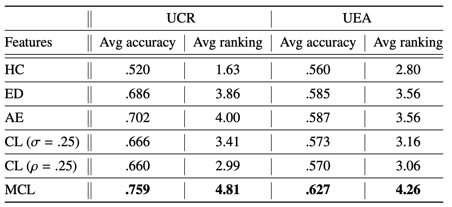
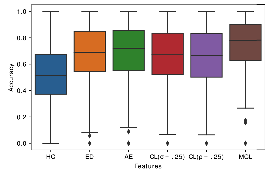
Accuracy & Ranking ( with 1-NN cls )

average across 5 training runs at the last epoch

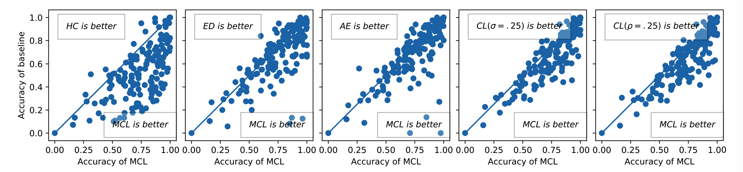
Accuracy ( scatter plot )

• diagonal = similar performance

Accuracy ( box plot )

• of UCR & UEA datasets

(2) Transfer Learning for clinical TS

Settings

• (1) classification of echocardiograms (ECGs) datasets
• (2) with limited datasets

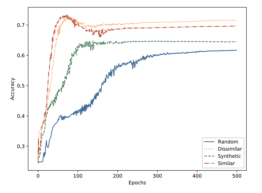
Process

• step 1) train an encoder
  • using MCL ( self-supervised pretext task )
  • pretext task datasets ( from UCR ) :
    • Syntehetic Control (Synthetic)
    • Swedish Leaf (Dissimilar)
    • ECG5000 (Similar)
• step 2) Initialize with pre-trained weights
  • ( encoder architecture : FCN )

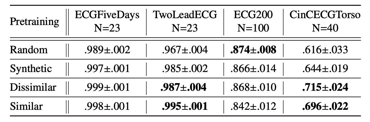
Accuracy

• Baseline : random initializatiion
• Proposed : 3 datasets
• ( \(N\) : number of training samples )

Accuracy ( by Epochs )