(paper 63) SSL for Semi-Supervised TSC

SSL for Semi-Supervised TSC

Contents

1. Abstract
2. Introduction
3. Method
   1. Forecasting as a SSL task
   2. MTL approach

0. Abstract

propose a new semi-supervised TSC model

• leverages features learned from the SSL task
• exploit the unlabeled training data with a forecasting task
• draw from established MTL approaches
  • main task : classification
  • auxiliary task : forecasting

1. Introduction

introduce MTL (Multi-task Learning)

• set of tasks is learned in parallel ( main and auxiliary tasks )
• auxiliary tasks : exist solely for the purpose of learning an enriched representation that could increase prediction accuracy over the main tasks

this paper uses “SSL + MTL”

• propose an auxiliary forecasting task
  • inherent in labeled and unlabeled time series data both. This

Step 1) define a sliding window function

• ( parameterized by stride & horizon to be forecasted )

Step 2) augment training set & generated samples

• for the forecasting task
• provide labeled & unlabeled samples as input

Step 3) ConvNet model is trained jointly,

• (1) to classify the labeled samples
• (2) to forecast future values

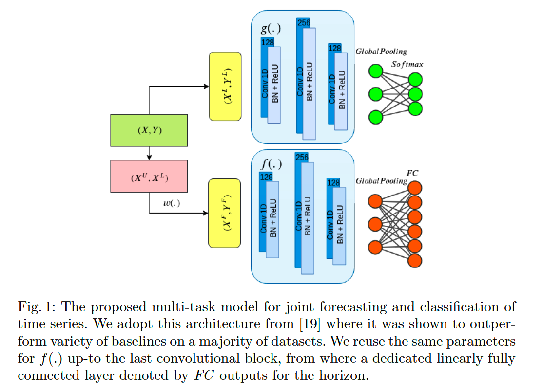
2. Method

Notation

• forecasting model : \(f(\cdot)\)
• classification model : \(g(\cdot)\)
• \(N\) univariate TS :
  • \(X=\left\{X_1, X_2, \ldots, X_n\right\}\).
  • \(Y=\left\{Y_1, Y_2, \ldots, Y_n\right\}\).

Split \(X\) ……. \(k+l=n\) &

• (labeled) \(X^L=\left\{X_1^L, X_2^L, \ldots, X_l^L\right\}\) & \(Y^L=\left\{Y_1^L, Y_2^L, \ldots, Y_l^L\right\}\)

• (unlabeled) \(\left\{X_1^U, X_2^U, \ldots, X_k^U\right\}\)

• \(k+l=n\) & total series length is \(T\).

Sliding window function \(w\)

• stride \(s\) and horizon \(h\)

• input : \(X\)
• output : segments of \(X\)
• ex) \(X_1\) ‘s first window :
  • \(X_{11}^F=\) \(\left\{x_{1, t=p}^1, x_{1, t=p+1}^1, \ldots, x_{1, t=p+h}^1\right\}\).
  • \(Y_{11}^F=\left\{y_{1, t=p+h+1}^1, y_{1, t=p+h+2}^1, \ldots, y_{1, t=p+2 h}^1\right\}\).
• next sample : chosen with regard to \(p=p+s\)
• result : \(X^F=\left\{X_{11}^F, X_{12}^F, \ldots, X_{n m}^F\right\}\) and \(Y^F=\left\{Y_1^F, Y_2^F, \ldots, Y_{n m}^F\right\}\)
• these windows have a total length of \(2 h<T\) of which the later half consists of targets to be forecasted
• # of forecasting samples, \(m=\) \(n \times\lfloor(2 \times h+1) / s\rfloor\)

Loss Function

• \(Y^F=f\left(X^F\right)\) and \(Y^L=g\left(X^L\right)\)
• \(L_f\left(X^F, \theta_f\right)=\frac{1}{n \times m \times h} \sum_i^n \sum_j^m \sum_t^h\left(y_{j t}^i-\hat{y}_{j t}^i\right)^2\).
  • model does multi-step predictions for the horizon \(h\)
• \(L_c\left(X^L, \theta_c\right)=-\frac{1}{l} \sum_i^l \log \left(\frac{e^{\hat{y}_{i=c}}}{\sum_j^C e^{\hat{y}_i}}\right)\).

(1) Forecasting as a SSL task

core intuition to model forecasting as an auxiliary task :

• force the ConvNet to learn a set of rich hidden state representations

• allows us flexibility in terms of data generation

  • By configuring the different values of the horizon and stride, \(h\) and \(s\) respectively

    \(\rightarrow\) can control the number of samples needed to configure an optimal balance between the classification and forecasting task samples

(2) MTL approach

2 key challenges :

• (1) how to divide the feature space in shared and task-specific
• (2) how to balance the weights between the different loss functions

This paper : hard parameter sharing

• learning parameters are all shared between the tasks up to the final FC layer

\(L_{M T L}\left(X^F, \theta_f, X^L, \theta_c\right)=L_c\left(X^L, \theta_c\right)+\lambda L_f\left(X^F, \theta_f\right)\).