(paper 78) MICN; Multi-Scale Local and Global Context Modeling for LTSF

MICN; Multi-Scale Local and Global Context Modeling for LTSF

Contents

1. Abstract
2. Introduction

0. Abstract

Transformer-based methods

• surprising performance in LTSF

Problem : attention mechanism for computing global correlations

• (1) entails high complexity

• (2) do not allow for targeted modeling of local features ( as CNN structures do )

Solution : propose to combine “LOCAL features & GLOBALcorrelations”

• to capture the overall view of time series (e.g., fluctuations, trends).

Multi-scale Isometric Convolution Network (MICN)

multi-scale branch structure is adopted

\(\rightarrow\) to model different potential patterns separately

• each pattern is extracted
  • (1) with down-sampled convolution : for LOCAL features
  • (2) with isometric convolution : for GLOBAL correlations

more efficient with linear complexity about the sequence length with suitable convolution kernels.

Experiments

• six benchmark datasets show that compared with state-of-the-art methods,
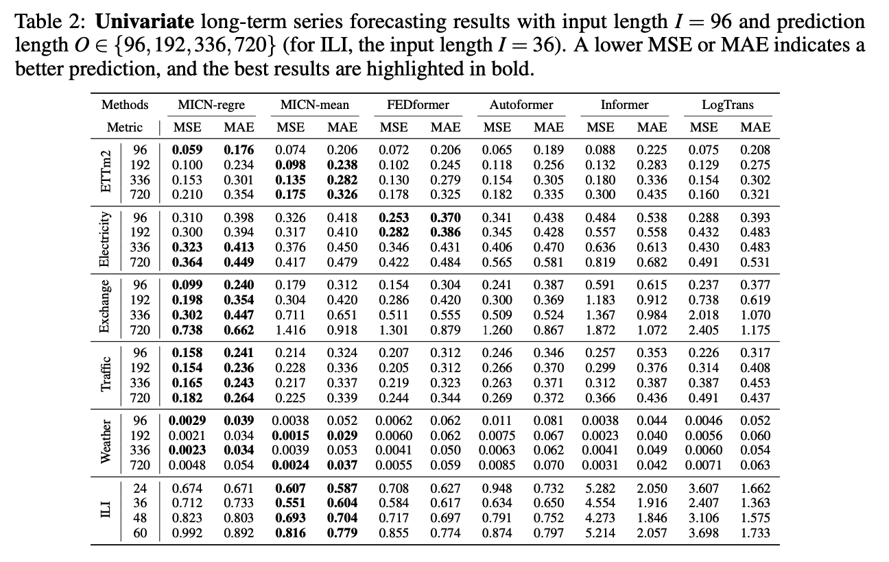
• yields 17.2% and 21.6% relative improvements for MTS & UTS

Code is available at https://github.com/wanghq21/MICN.

1. Introduction

LTSF (Long-term Time Series Forecasting)

• input : \(X_1, X_2, \ldots, X_{t-1}, X_t\)
• target : \(X_{t+1}, X_{t+2}, \ldots, X_{t+T-1}, X_{t+T}\)

where \(T \gg t\).

CNN-based method

TCN (Bai et al., 2018)

• (1) causal convolution
  • to model the temporal causality
• (2) dilated convolution
  • to expand the receptive field.

\(\rightarrow\) can integrate the local information of the sequence better & achieve competitive results in short/medium-term forecasting

However, limited by the receptive field size, TCN often needs many layers to model the global relationship of time series

Transformer-based method

Pros

• Can model the long-term dependence of sequences effectively,

• Learned attention matrix

  • represents the correlations between different time points of the sequence
  • can explain relatively well how the model makes future predictions based on past information.

Cons

• has a quadratic complexity

  ( + many of the computations between token pairs are non-essential )

  \(\rightarrow\) interesting research direction to reduce its computational complexity.

Examples )

• LogTrans (Li et al., 2019b)
• Informer (Zhou et al., 2021)
• Reformer (Kitaev et al., 2020)
• Autoformer Wu et al. (2021b)
• Pyraformer (Liu et al., 2021a)
• FEDformer (Zhou et al., 2022)

This paper: combine the modeling perspective of CNNs with that of Transformers

• to build models from the realistic features of the sequences themselves,

  ( i.e., LOCAL features and GLOBAL correlations )

• Local features
  • represent the characteristics of a sequence over a small period \(T\)
• Global correlations
  • correlations exhibited between many periods \(T_1, T_2, \ldots T_{n-1}, T_n\).

2 properties of good forecasting method

• (1) The ability to extract LOCAL features to measure short-term changes.
• (2) The ability to model the GLOBAL correlations to measure the long-term trend.

Multi-scale Isometric Convolution Network (MICN)

Use multiple branches of different convolution kernels to model different potential pattern information of the sequence separately.

each branch :

• ( bottom ) extract the local features of the sequence using a local module based on downsampling convolution
• ( top ) model the global correlation using a global module based on isometric convolution

Merge operation

• to fuse information about different patterns from several branches.

\(\rightarrow\) reduces the time & space complexity to linearity,

Contribution

• (1) propose MICN based on convolution structure
  • to efficiently replace the self-attention
  • achieves linear computational complexity and memory cost.
• (2) propose a multiple branches framework
• (3) propose a local-global structure
  • to implement information aggregation and long-term dependency modeling for TS
  • for local featurer extraction : downsampling one-dimensional convolution
  • for global correlations : isometric convolution

2. Related Work

(1) CNNs & Transformers

CNN-based methods

• usually modeled from the local perspective

• convolution kernels are good at extracting local information

• By continuously stacking CNN layers…

  \(\rightarrow\) the field of perception can be extended to the entire input space

Transformer

• attention mechanism

• Unlike modeling local information directly from the input, does not require stacking many layers to extract global information.

• pros & cons
  • pros) more capable of learning long-term dependencies
  • cons) complexity is higher and learning is more difficult

Although CNNs and Transformers are modeled from different perspectives,

they both aim to achieve efficient utilization of the overall information of the input.

[ Summary ]

This paper : to combine CNNs & Transformemrs…

• consider both local and global context
  • step 1) extract local features
  • step 2) model global correlation on this basis.
• achieves lower computational effort and complexity.

(2) Modeling Both Local and Global Context

Studies on how to combine local and global modeling into a unified model to achieve high efficiency and interpretability

a) Conformer (Gulati et al., 2020)

Used in many speech applications.

Architecture

• Attention mechanism to learn the global interaction,

• Convolution module to capture the relative-offset-based local features

\(\rightarrow\) combines these two modules sequentially.

Problems?

• (1) does not analyze in detail what local and global features are learned and how they affect the final output.

• (2) no explanation why the attention module is followed by a convolution module.
• (3) quadratic complexity w.r.t sequence length

b) Lite Transformer (Wu et al., 2020)

Architecture (similar)

• Attention mechanism to capture long-term correlation

• Convolution module to capture local information

\(\rightarrow\) combines these two modules sequentially.

but it separates them into two branches for parallel processing.

+ visual analysis of the feature weights extracted from the two branches

Problem

• (1) parallel structure of the two branches

  \(\rightarrow\) may be some redundancy in its computation,

• (2) limitation of quadratic complexity.

c) Proposed method

New framework for modeling local features and global correlations,

using new module instead of attention mechanism.

• use the convolution operation to extract its local information
• use the isometric convolution to model the global correlation between each segment of the local features.

Not only avoids more redundant computations

& also reduces the overall time and space complexity to linearity w.r.t squence length

3. Model

(1) MICN Framework

LTSF task

• target : future series of length \(O\)
• input : past series of length \(I\),

where \(O\) is much larger than \(I\).

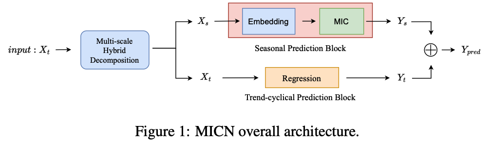
Overview

(1) Multi-scale hybrid decomposition (MHDecomp) block

• to separate complex patterns of input series.

(2) Seasonal Prediction Block

• to predict seasonal information

(3) Trend-cyclical Prediction Block

• to predict trend-cyclical information.

\(\rightarrow\) Then add the prediction results up to get the final prediction \(Y_{\text {pred }}\).

• \(d\) : number of variables in MTS
• \(D\): number of variables in the hidden state of the series.

(2) Multi-scale hybrid decomposition (MHDecomp)

Previous series decomposition algorithms

• MA to smooth out periodic fluctuations

• For input series \(X \in R^{I \times d}\)

  • [Trend] \(X_t =\operatorname{AvgPool}(\text { Padding }(X))_{k e r n e l}\).
  • [Seasonality] \(X_s =X-X_t\)

• use of the \(\operatorname{Avg} \operatorname{pool}(\cdot)\) with the padding operation

  \(\rightarrow\) keeps the series length unchanged.

• Problem : large differences in trend-cyclical series and seasonal series obtained from different kernels.

Multi-scale hybrid decomposition block

• uses several different kernels of the \(\operatorname{Avg} \operatorname{pool}(\cdot)\)

• separate several different patterns of TREND-cyclical and SEASONAL parts

• ( Different from the MOEDecomp block of FEDformer )

  • use simple mean operation to integrate these different patterns

    ( because we cannot determine the weight of each pattern )

  • put this weighting operation in the Merge part of Seasonal Prediction block after the representation of the features.

• For input series \(X \in R^{I \times d}\)

  • [Trend] \(X_t=\operatorname{mean}\left(\operatorname{AvgPool}(\operatorname{Padding}(X))_{\text {kernel }_1}, \ldots, \operatorname{AvgPool}(\operatorname{Padding}(X))_{\text {kernel }_n}\right)\)
  • [Seasonality] \(X_s=X-X_t\)

• different kernels are consistent with multi-scale information in Seasonal Prediction block.

(3) Trend-cyclical Prediction Block

Autoformer (Wu et al., 2021b)

• concatenates the mean of the original series
• accumulates it with the trend-cyclical part

\(\rightarrow\) no proof of its effectiveness.

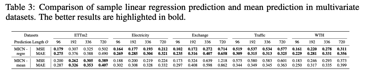
This paper

• use a simple linear regression strategy to make a prediction about trend-cyclical
• demonstrate that simple modeling of trend-cyclical is also necessary for non-stationary series forecasting tasks (See Section 4.2).
• Trend-cyclical series \(X_t \in R^{I \times d}\) :
  • \(Y_t^{\text {regre }}=\text { regression }\left(X_t\right)\).
    • where \(Y_t^{\text {regre }} \in R^{O \times d}\)
    • denotes the prediction of the trend part
• For comparison, we use the mean of \(X_t\) to cope with the series where the trend-cyclical keeps constant
• \(Y_t^{\text {mean }}=\operatorname{mean}\left(X_t\right)\).

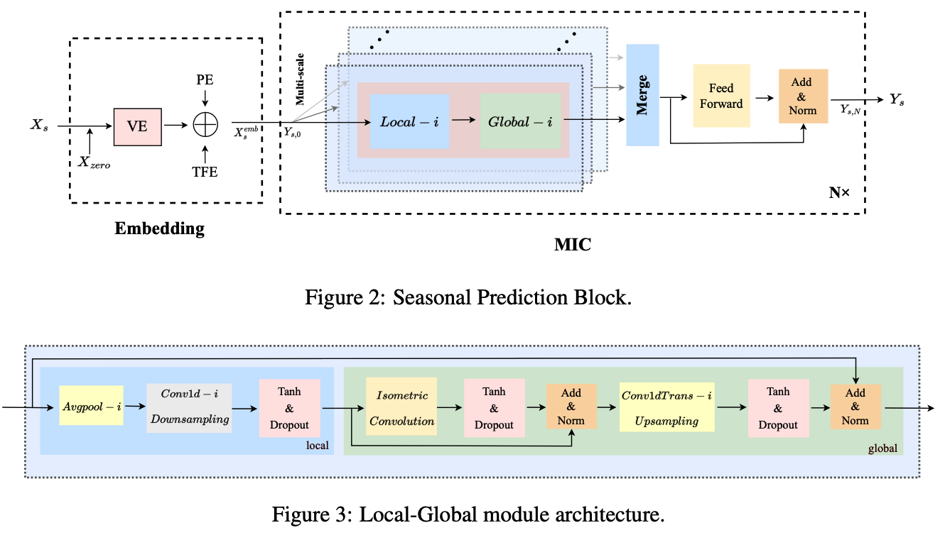
(4) Seasonal Prediction Block

focuses on the more complex seasonal part modeling.

• step1) embed the input sequence \(X_s\),
• step 2) adopt multi-scale isometric convolution
  • to capture the local features and global correlations,
  • branches of different scales model different underlying patterns
• step 3) merge the results from different branches

Summary :

\[\begin{aligned} X_s^{e m b} & =\operatorname{Embedding}\left(\operatorname{Concat}\left(X_s, X_{\text {zero }}\right)\right) \\ Y_s^0 & =X_s^{\text {emb }} \\ Y_{s, l} & =M I C\left(Y_{s, l-1}\right), \quad l \in\{1,2, \ldots, N\} \\ Y_s & =\operatorname{Truncate}\left(\operatorname{Projection}\left(Y_{s, N}\right)\right), \end{aligned}\]

Notation :

• \(X_{\text {zero }} \in R^{O \times d}\) : the placeholders filled with zero
• \(X_s^{\text {emb }} \in R^{(I+O) \times D}\) : the embedded representation of \(X_s\)
• \(Y_{s, l} \in R^{(I+O) \times D}\) : the output of \(l-t h\) multi-scale isometric convolution (MIC) layer
• \(Y_s \in R^{O \times d}\) : final prediction of the seasonal part after
  • linear function Projection with \(Y_{s, N} \in R^{(I+O) \times D}\)
  • and Truncate operation

a) Embedding

Decoder of Informer / Autoformer / Fedformer

• contain the latter half of the encoder’s input with the length \(\frac{I}{2}\) and placeholders with length \(\mathrm{O}\) filled by scalars,

  \(\rightarrow\) may lead to redundant calculations.

Solution : replace (1) \(\rightarrow\) (2)

• (1) traditional encoder-decoder style input
• (2) simpler complementary 0 strategy.

Follow the setting of FEDformer & adopt three parts to embed the input

• \(X_s^{\text {emb }}=\operatorname{sum}\left(T F E+P E+V E\left(\text { Concat }\left(X_s, X_{\text {zero }}\right)\right)\right)\).

  • where \(X_s^{e m b} \in R^{(I+O) \times D}\).

  • (1) \(TFE\) : time features encoding

    ​ (e.g., MinuteOfHour, HourOfDay, DayOfWeek, DayOfMonth, and MonthOfYear)

  • (2) \(P E\) : positional encoding

  • (3) \(V E\) : value embedding.

b) Multi-scale isometric Convolution(MIC) Layer

contains several branches

• with different scale sizes
  • used to model potentially different temporal patterns.
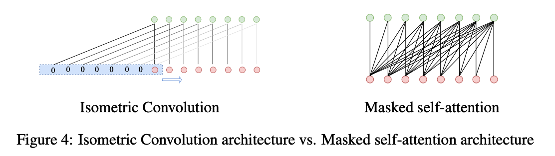
• Each branch : local-global module

Local Module

• after obtaining the corresponding single pattern by avgpool …
• adopts 1D-conv to implement downsampling.

Notation

• \(Y_{s, l} =Y_{s, l-1}\).
• \(Y_{s, l}^{\text {local }, i} =\operatorname{Conv1d}\left(\operatorname{Avgpool}\left(\operatorname{Padding}\left(Y_{s, l}\right)\right)_{\text {kernel=i }}\right)_{\text {kernel }=i}\).
  • \(Y_{s, l-1}\) : the output of \((l-1)-t h\) MIC layer
  • \(Y_{s, 0}=X_s^{e m b} . i \in\left\{\frac{I}{4}, \frac{I}{8}, \ldots\right\}\) : the different scale sizes corresponding to the different branches
  • \(Y_{s, l}^{\text {local,i }} \in R^{\frac{(I+O)}{i} \times D}\) : results obtained by compressing local features ( = short sequence )

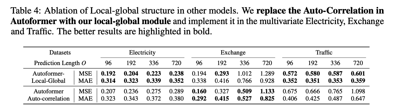
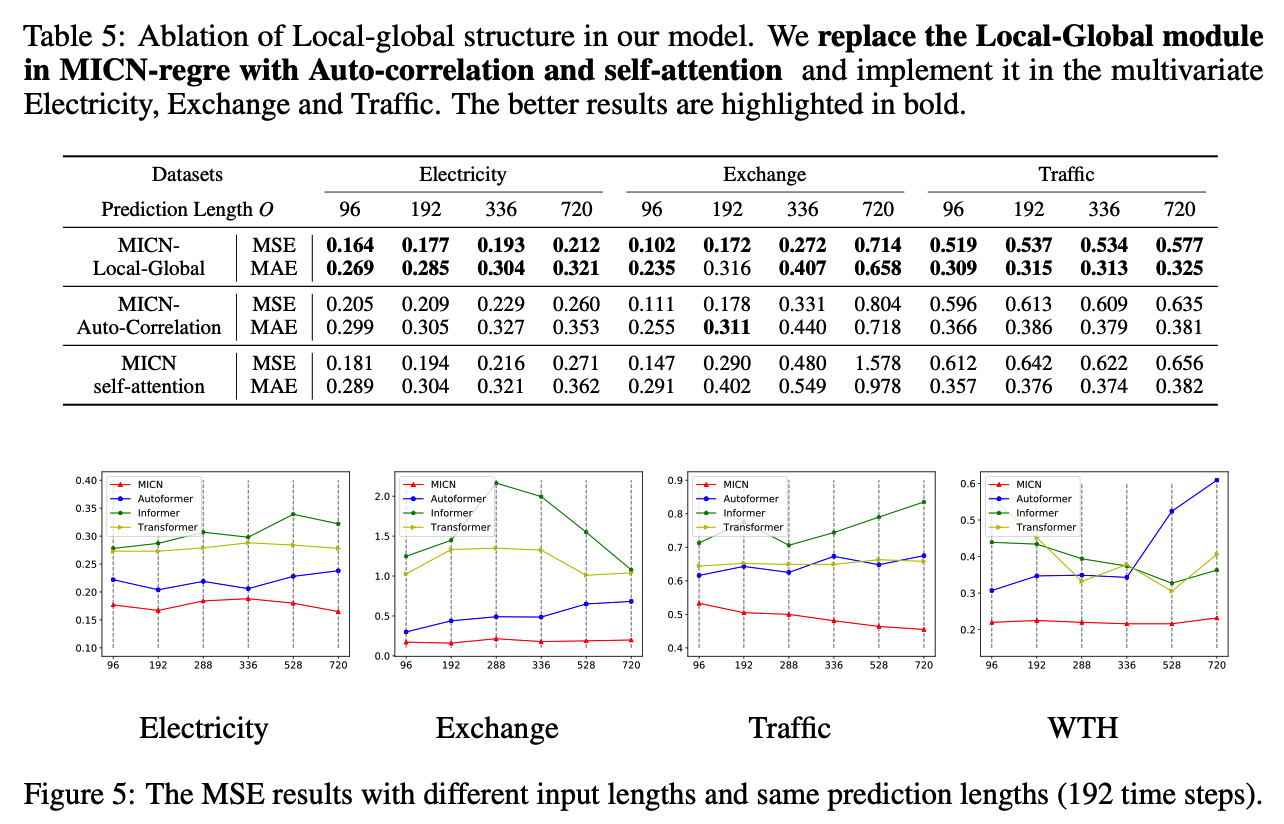
Global Module

• to model the global correlations of the output of the local module
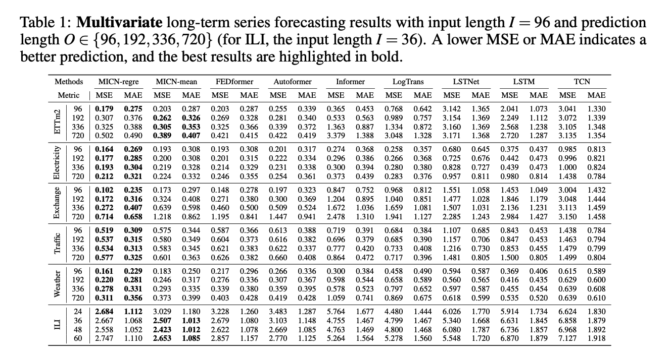
• self-attention mechanism (X)
• use a variant of casual convolution, isometric convolution (O)

Isometric convolution??

• pads the sequence of length \(S\), with placeholders zero of length \(S-1\)
• Kernel size = \(S\)

\(\rightarrow\) can use large kernel size !!

Previous works

• add placeholder to the input sequence

  ( = which has no actual sequence information in the second half )

Isometric Convolution

• enable sequential inference of sequences by fusing local features information.
• kernel of Isometric convolution is determined by all the training data
  • can introduces a global temporal inductive bias
  • achieve better generalization than self-attention
• + for a shorter sequence, isometric convolution is superior to self-attention.

Notation

• \(Y_{s, l}^{\prime, i} =\operatorname{Norm}\left(Y_{s, l}^{l o c a l, i}+\operatorname{Dropout}\left(\operatorname{Tanh}\left(\operatorname{IsometricConv}\left(Y_{s, l}^{l o c a l, i)}\right)\right)\right)\right.\).
• \(Y_{s, l}^{\text {global }, i} =\operatorname{Norm}\left(Y_{s, l-1}+\operatorname{Dropout}\left(\operatorname{Tanh}\left(\operatorname{Conv} 1 \operatorname{dranspose}\left(Y_{s, l}^{\prime, i}\right)_{\text {kernel=i }}\right)\right)\right)\).
  • \(Y_{s, l}^{l o c a l, i} \in R^{\frac{(I+O)}{i} \times D}\) : the result after the global correlations modeling
  • \(Y_{s, l-1}\) : output of \(l-1\) MIC layer
  • \(Y_{s, l}^{\text {global }, i} \in R^{(I+O) \times D}\) : the result of this pattern (i.e., this branch).

Merge

• use Conv2d to merge different patterns
• with different weights ( not concatenate )

Notation

• \(Y_{s, l}^{\text {merge }} =\left(\operatorname{Conv} 2 d\left(Y_{s, l}^{\text {global }, i}, i \in\left\{\frac{I}{4}, \frac{I}{8}, \ldots\right\}\right)\right)\).
• \(Y_{s, l} =\operatorname{Norm}\left(Y_{s, l}^{\text {merge }}+\text { FeedForward }\left(Y_{s, l}^{\text {merge }}\right)\right)\).
  • \(Y_{s, l} \in R^{(I+O) \times D}\) : the result of \(l-t h\) MIC layer.

Final prediction

• use the projection and truncate operations:

• \(Y_s=\operatorname{Truncate}\left(\operatorname{Projection}\left(Y_{s, N}\right)\right)\).

  • \(Y_{s, N} \in R^{(I+O) \times D}\) : the output of \(\mathrm{N}\)-th MIC layer
  • \(Y_s \in R^{O \times d}\) : the final prediction about the seasonal part.

4. Experiments

(1) Main Results

(2) Ablation Studies