ScaleFormer: Iterative Multi-scale Refining Transformers for TS Forecasting
Contents
- Abstract
- Introduction
- Method
- Problem Setting
- Multi-scale Framework
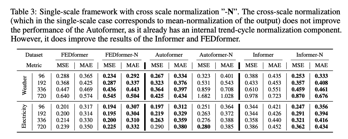
- Cross-scale Normalization
- Input Embedding
- Loss Function
- Experiments
- Main Results
- Ablation Study
- Qualitative Comparison
0. Abstract
Propose a general multi-scale framework
- that can be applied to the transformer-based TS forecasting models
(1) Iteratively refine a forecasted time series at multiple scales with shared weights,
(2) Introduce architecture adaptations & a specially-designed normalization scheme
\(\rightarrow\) achieve significant performance improvements
( with minimal additional computational overhead. )
1. Introduction
Integrating information at different time scales is essential
Transformer-based architectures have become the mainstream
Advances have focused mainly on mitigating the standard quadratic complexity in time and space, rather than explicit scale-awareness.
-
The essential cross-scale feature relationships are often learnt implicitly,
( not encouraged by architectural priors of any kind )
Autoformer & Fedformer
-
introduced some emphasis on scale-awareness
( by enforcing different computational paths for the trend and seasonal components of the input time series )
-
However, this structural prior only focused on two scales: low & high-frequency components.
Can we make transformers more scale-aware?
\(\rightarrow\) Scaleformer
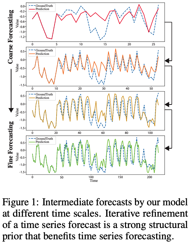
Time series forecasts are iteratively refined at successive time-steps,
\(\rightarrow\) allow the model to better capture the inter-dependencies and specificities of each scale
However, scale itself is not sufficient.
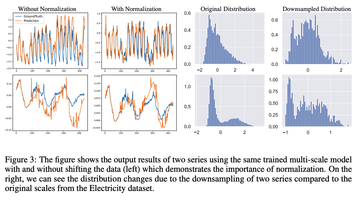
Iterative refinement at different scales can cause significant distribution shifts between intermediate forecasts, which can lead to runaway error propagation
\(\rightarrow\) introduce cross-scale normalization at each step
Proposed work
-
re-orders model capacity to shift the focus on scale awareness
( does not fundamentally alter the attention-driven paradigm of transformers )
-
can be readily adapted to work jointly wit SOTA transformers
( acting broadly orthogonally to their own contributions )
- e.g. Fedformer, Autoformer, Informer, Reformer, Performer
Contributions
(1) Introduce a novel iterative scale-refinement paradigm
- can be readily adapted to a variety of transformer-based methods
(2) Introduce cross-scale normalization on outputs of the Transformer
- To minimize distribution shifts between scales and windows
2. Method
(1) Problem Setting
Notation
- \(\mathbf{X}^{(L)}\) : look-back windows ( length = \(\ell_L\) )
- \(\mathbf{X}^{(H)}\) : horizon windows ( length = \(\ell_H\) )
- time-series of dimension \(d_x\) :
- \(\mathbf{X}^{(L)}=\left\{\mathbf{x}_t \mid \mathbf{x}_t \in \mathbb{R}^{d_x}, t \in\left[t_0, t_0+\ell_L\right]\right\}\).
- \(\mathbf{X}^{(H)}=\left\{\mathbf{x}_t \mid \mathbf{x}_t \in \mathbb{R}^{d_x}, t \in\left[t_0+\ell_L+\right.\right. \left.\left.1, t_0+\ell_L+\ell_H\right]\right\}\).
Goal :
- predict the horizon window \(\mathbf{X}^{(H)}\) given the look-back window \(\mathbf{X}^{(L)}\).
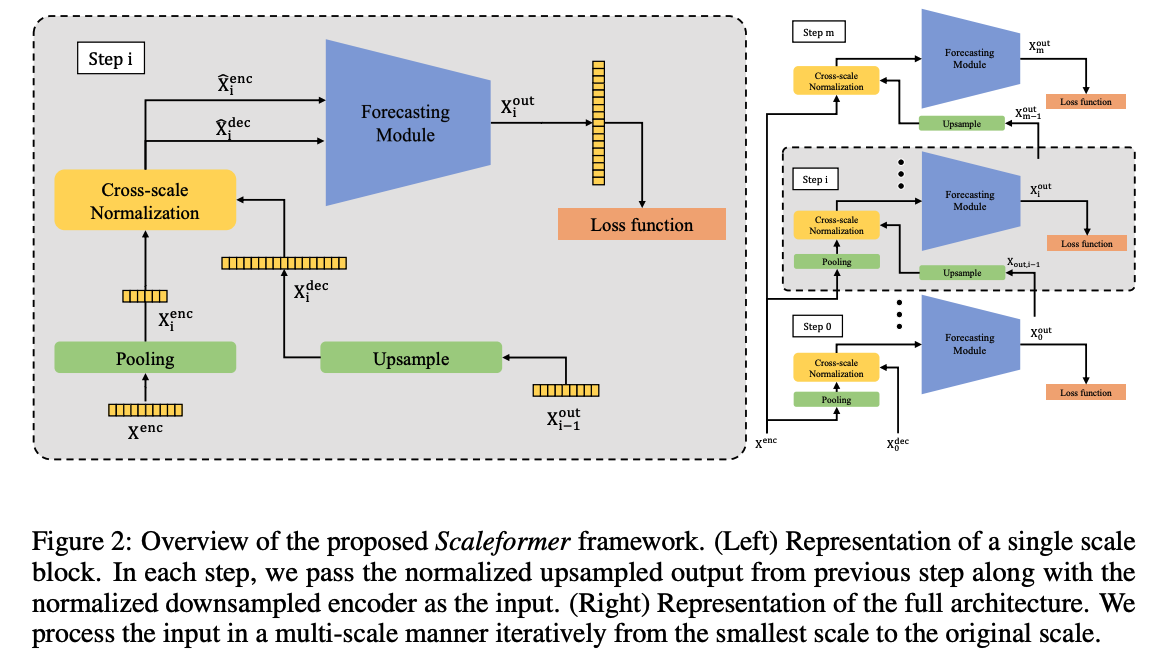
(2) Multi-scale Framework
applies successive transformer modules to iteratively refine a time-series forecast, at different temporal scales
Details :
-
given an input time-series \(\mathbf{X}^{(L)}\) ….
iteratively apply the same neural module mutliple times at different temporal scales.
-
set of scales \(S=\left\{s^m, \ldots, s^2, s^1, 1\right\}\)
- (i.e. for the default scale of \(s=2, S\) is a set of consecutive powers of 2)
- where \(m=\left\lfloor\log _s \ell_L\right\rfloor-1\) and \(s\) is a downscaling factor.
Input to …
- (encoder) at the \(i\)-th step \((0 \leq i \leq m)\) : the original look-back window \(\mathbf{X}^{(L)}\),
- downsampled by a scale factor of \(s_i \equiv s^{m-i}\) via an average pooling operation.
- (decoder) : \(\mathbf{X}_{i-1}^{\text {out }}\) upsampled by a factor of \(s\) via a linear interpolation.
- \(\mathbf{X}_0^{\text {dec }}\) is initialized to an array of 0s
Loss : error between \(\mathbf{X}_i^{(H)}\) and \(\mathbf{X}_i^{\text {out }}\)
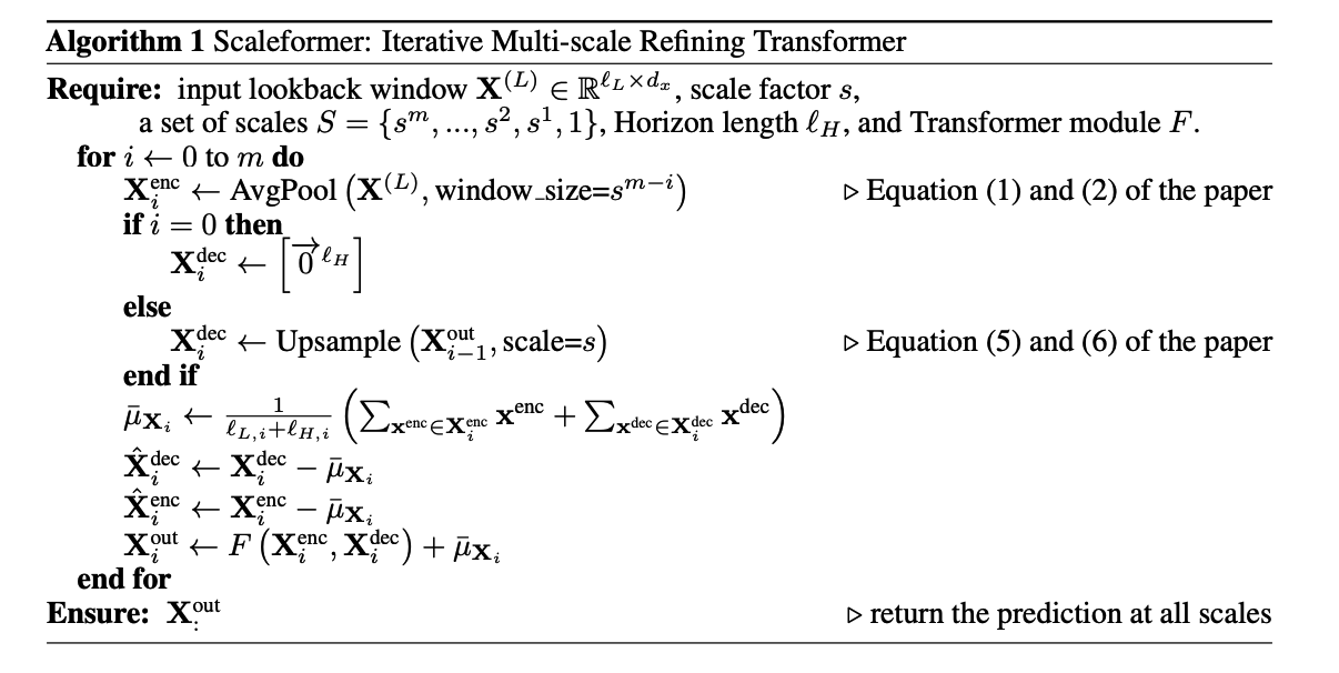
(3) Cross-scale Normalization
Input series \(\left(\mathbf{X}_i^{\mathrm{enc}}, \mathbf{X}_i^{\text {dec }}\right)\),
- with dimensions \(\ell_{L_i} \times d_x\) and \(\ell_{H_i} \times d_x\), respectively
Normalize each series
- based on the temporal average of \(\mathbf{X}_i^{\mathrm{enc}}\) and \(\mathbf{X}_i^{\text {dec }}\).
- \(\begin{aligned}
\bar{\mu}_{\mathbf{X}_i} & =\frac{1}{\ell_{L, i}+\ell_{H, i}}\left(\sum_{\mathbf{x}^{\text {enc }} \in \mathbf{X}_i^{\mathrm{enc}}} \mathbf{x}^{\mathrm{enc}}+\sum_{\mathbf{x}^{\mathrm{dec}} \in \mathbf{X}_i^{\mathrm{dec}}} \mathbf{x}^{\mathrm{dec}}\right) \\
\hat{\mathbf{X}}_i^{\mathrm{dec}} & =\mathbf{X}_i^{\mathrm{dec}}-\bar{\mu}_{\mathbf{X}_i}, \quad \hat{\mathbf{X}}_i^{\mathrm{enc}}=\mathbf{X}_i^{\mathrm{enc}}-\bar{\mu}_{\mathbf{X}_i}
\end{aligned}\).
- \(\bar{\mu}_{\mathbf{X}_i} \in \mathbb{R}^{d_x}\) : average over the temporal dimension of the concatenation of both look-back window and the horizon.
- \(\hat{\mathbf{X}}_i^{\text {enc }}\) and \(\hat{\mathbf{X}}_i^{\text {dec }}\) : inputs of the \(i\) th step to the forecasting module.
Distribution shift
- distribution of input to a model changes across training to deployment
- two distinct distribution shifts
- (1) Covariate shift
- natural distribution shift between the look-back & forecast window
- (2) Shift between the predicted forecast windows at two consecutive scales
- which is a result of the upsampling operation
- (1) Covariate shift
\(\rightarrow\) Normalizing the output at a given step by either the look-back window statistics or the previously predicted forecast window statistics result in an accumulation of errors across steps.
\(\rightarrow\) Mitigate this by considering a moving average of forecast and look-back statistics as the basis for the output normalization
(4) Input Embedding
skip
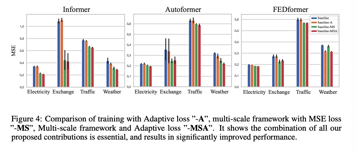
(5) Loss function
Using the standard MSE objective
\(\rightarrow\) sensitive to outliers.
Thus, use objectives more robust to outliers
- ex) Huber loss (Huber, 1964).
However, when there are no major outliers, such objectives tend to underperform
\(\rightarrow\) instead, utilize adaptive loss
\(f(\xi, \alpha, c)=\frac{ \mid \alpha-2 \mid }{\alpha}\left(\left(\frac{(\xi / c)^2}{ \mid \alpha-2 \mid }+1\right)^{\alpha / 2}-1\right)\).
## (2) Ablation Study 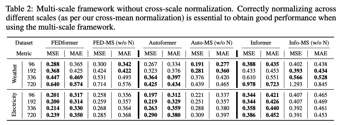
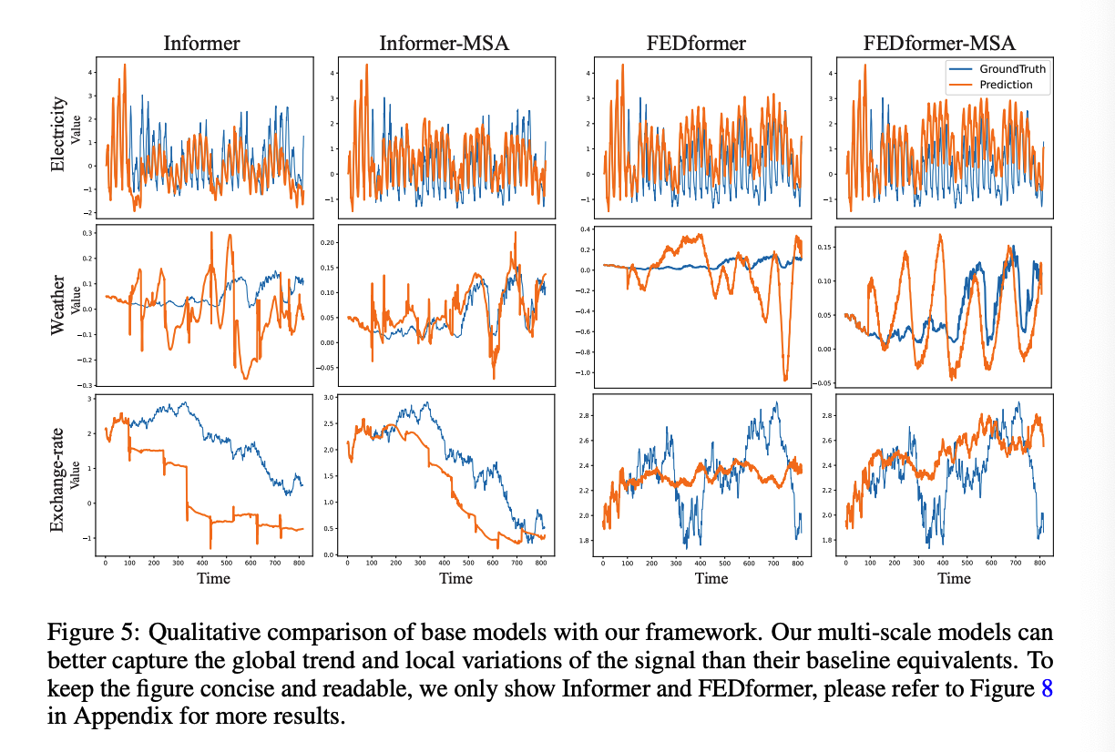
## (3) Qualitative Comparison