
CAN: A Simple, Efficient and Scalable CMAE framework for learning Visual Representations
( https://openreview.net/forum?id=qmV_tOHp7B9 )
Contents
- Abstract
- Introduction
- Manifold Mixup
- Manifold Mixup Flattens Representations
0. Abstract
CAN : minimal and conceptually clean synthesis of ..
- (C) contrastive learning
- (A) masked autoencoders
- (N) noise prediction approach used in diffusion models
complementary to one another:
(C) contrastive learning
- shapes the embedding space across a batch of image samples
(A) masked autoencoders
- focus on reconstruction of the low-frequency spatial correlations in a single image sample
(N) noise prediction
- encourages the reconstruction of the high-frequency components of an image
\(\rightarrow\) combination : robust, scalable and simple-to-implement algorithm.
1. A Simple CMAE framework
3 different objectives
- (1) contrastive
- (2) reconstruction
- (3) denoising.
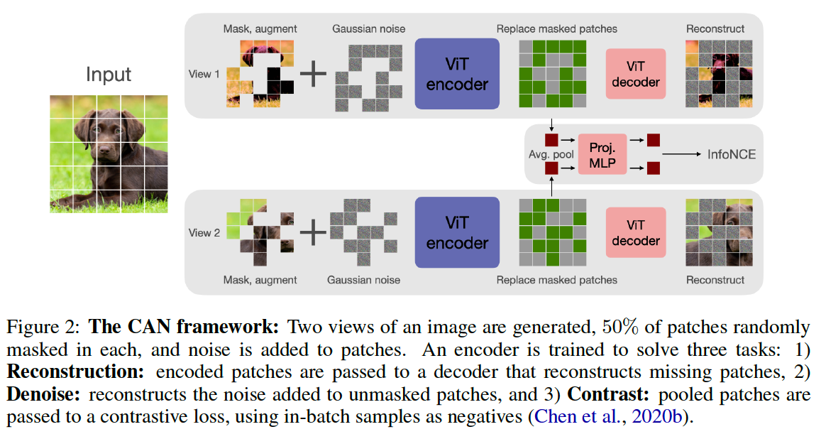
(1) Overview
Batch of \(n\) images \(\{\mathbf{x}\}_{i=1}^n\)
- 2 views : \(\mathbf{x}_i^1, \mathbf{x}_i^2 \in \mathbb{R}^{h \times w \times 3}\) of each image
- Each image is then split into \(T=(h / p) \times(w / p)\) patches of size \(p \times p\)
- \[\mathbf{x}_{i, \text { patch }}^1, \mathbf{x}_{i, \text { patch }}^2 \in \mathbb{R}^{T \times p \times p \times 3}\]
Two masks : \(\mathbf{M}_i^1, \mathbf{M}_i^2 \in\) \(\{0,1\}^T\)
-
1 = masked & 0 = unmasked
- coordinate \(t \in\{1, \ldots T\}\)
- unmasked with probability \(m\)
- default masking rate is \(m=50 \%\)
- (for MAE we use the default \(75 \%\) ).
only the \(T^{\prime}\) unmasked patches are passed to the ViT encoder
- Masking a large fraction of patches from both views make our method much more efficient than contrastive methods that use two full views
collect the embeddings of unmasked tokens \(\mathbf{z}_i^1, \mathbf{z}_i^2 \in \mathbb{R}^{T^{\prime} \times d}\)
& add with learned \([\mathrm{M}]\) embedding to positions corresponding to masked tokens.
\(\rightarrow\) reshape into \(T \times d\) tensors
\(\rightarrow\) then passed through a comparatively lightweight ViT decoder
- produce outputs \(\hat{\mathbf{x}}_i^1, \hat{\mathbf{x}}_i^2\) in image space \(\mathbb{R}^{h \times w \times 3}\).
(2) [C] Contrastive Learning Objective
Embeddings \(\mathbf{z}_i^1, \mathbf{z}_i^2 \in \mathbb{R}^{T^{\prime} \times d}\) ( = output of encoder )
\(\rightarrow\) pooled via a simple mean ( along the first dimension ) … form \(d\)-dim embeddings
\(\rightarrow\) passed through a lightweight MLP projection head that maps into a lower dim \(\mathbb{R}^r, r<d\),
\(\rightarrow\) normalized to unit length
- output : embeddings \(\mathbf{u}_i^1, \mathbf{u}_i^2 \in \mathbb{R}^r\) for \(i=1, \ldots n\).
Example ) negative of \(i\)-th item :
- other \(2 n-2\) samples in-batch \(\mathcal{N}_i=\left\{\mathbf{u}_j^1, \mathbf{u}_j^2\right\}_{j \neq i}\)
InfoNCE loss : \(\mathcal{L}_{\text {InfoNCE }}=\frac{1}{2 n} \sum_{v=1,2} \sum_{i=1}^n-\log \frac{e^{\mathbf{u}_i^{1 \top} \mathbf{u}_i^2 / \tau}}{e^{\mathbf{u}_i^{1_i^{\top}} \mathbf{u}_i^2 / \tau}+\sum_{\mathbf{u}^{-} \in \mathcal{N}_i} e^{\mathbf{u}_i^{v \top} \mathbf{u}^{-} / \tau}}\).
- set to \(\tau=0.1\) by default
(3) [A] Patch Reconstruction Objective
\(\hat{\mathbf{x}}_i^1, \hat{\mathbf{x}}_i^2\) : outputs of ViT decoder
Trained to reconstruct the missing patches of each image.
Compute the reconstruction loss only on masked patches
- \(\mathcal{L}_{\mathrm{rec}}=\frac{1}{2 n} \sum_{v=1,2} \sum_{i=1}^n \mid \mid \mathbf{M}_i^v \circ\left(\mathbf{x}_i^v-\hat{\mathbf{x}}_i^v\right) \mid \mid _2^2\).
Computing the loss only on masked patches gives better performance …
\(\rightarrow\) indicates wasted computation since the decoder also produces reconstructions for unmasked patches
\(\rightarrow\) to avoid waste … propose an alternative objective specifically for “unmasked” patches
(4) [N] Denoising Objective
Inspired by diffusion modelling using denoising training objectives & score-based counterparts
\(\rightarrow\) revisit the suitability of denoising for self-supervised learning.
Add independent isotropic Gaussian noise to each image
- \(\mathbf{x}_i^v \leftarrow \mathbf{x}_i^v+\sigma_i^v \mathbf{e}_i^v\) with \(\mathbf{e}_i^v \sim \mathcal{N}(\mathbf{0}, I)\) and \(\sigma_i^v\) uniformly sampled from \(\left[0, \sigma_{\max }\right]\)
Details
-
provide the decoder with information on the noise level \(\sigma_i^v\)
( to help it separate noise from the GT image )
-
motivated by denoising diffusion methods
- pass both the noisy image & noise level as inputs to the denoising model
- achieve this by using \(\sigma_i^v\) as a positional encoding in the decoder
Step 1) produce a sinusoidal embedding of \(\sigma_i^v \in \mathbb{R}^d\)
Step 2) passed through a lightweight 2 layer MLP with ReLU activations
- produce a (learnable) embedding \(\mathbf{p}_i^v \in \mathbb{R}^d\),
- dim = same as \(\mathbf{z}_i^v \in \mathbb{R}^{T \times d}\).
Step 3) add \(\mathbf{p}_i^v \in \mathbb{R}^d\) to each embedded token ( & missing tokens \([\mathrm{M}]\) )
-
to provide noise-level information
-
\(\left(\mathbf{z}_i^v\right)_t \leftarrow\left(\mathbf{z}_i^v\right)_t+\mathbf{p}_i^v\) for \(t=1 \ldots, T\),
Step 4) pass the result to the decoder to produce \(\mathbf{x}_i^v\).
Loss Function
- computed only on unmasked pixels
- \(\mathcal{L}_{\text {denoise }}=\frac{1}{2 n} \sum_{v=1,2} \sum_{i=1}^n \mid \mid \left(1-\mathbf{M}_i^v\right) \circ\left(\sigma_i^v \mathbf{e}_i^v-\hat{\mathbf{x}}_i^v\right) \mid \mid _2^2\).