(강의) SVM & KKT

Optimization in Unsupervised Learning

Contents

1. Introduction

1. Introduction

(1) Unsupervised Learning이란

\(X = (x_1 , \cdots x_m )\) where \(x_i \in R^{n}\)

• NO LABEL!!

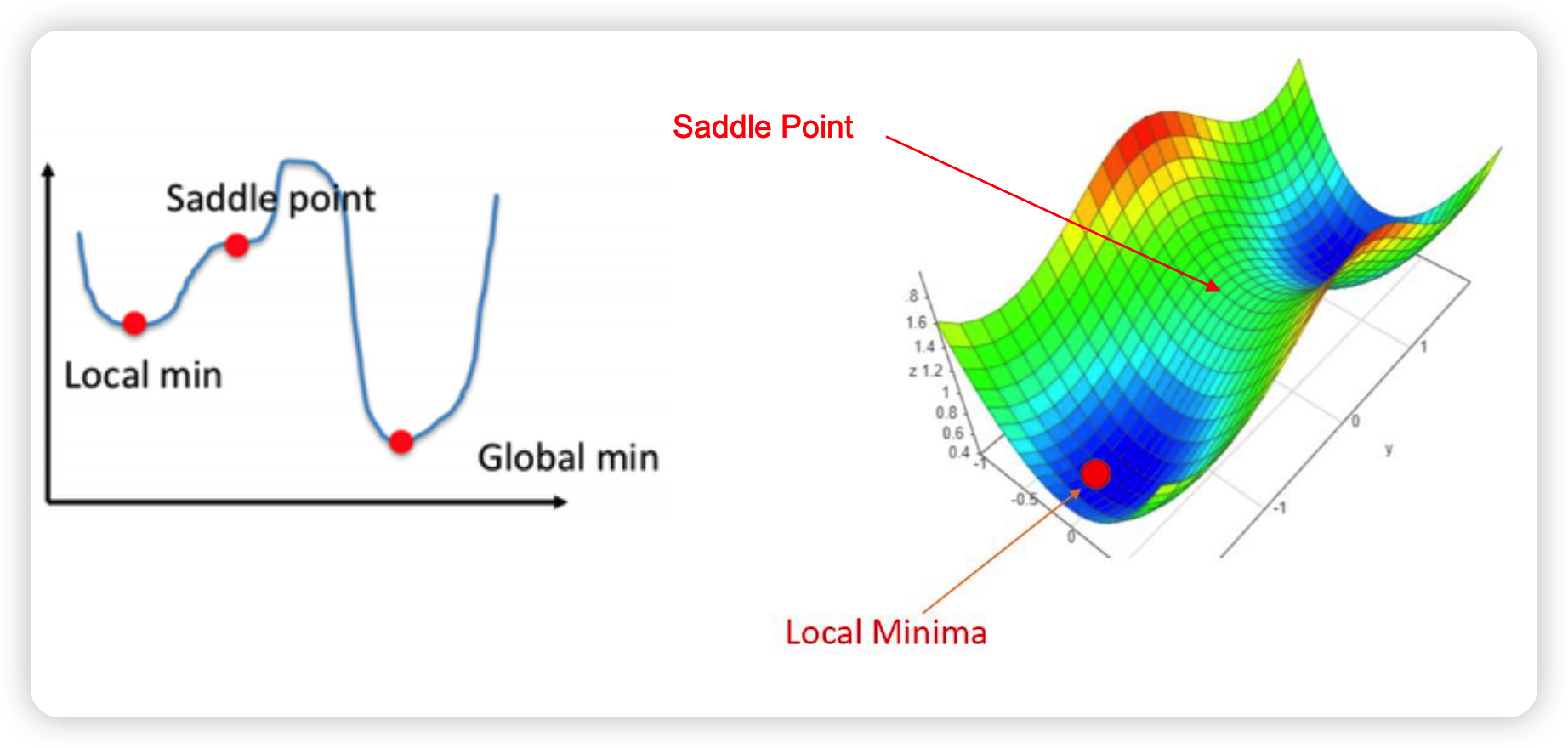
(2) Non-convex optimization

KKT condition은 “LOCAL min.max”를 보장하지, “GLOBAL”은 보장하지 않는다.

2. Example of non-convex opt

a) SPARSE linear regression

\(\begin{aligned} &\min _{w} f(w)= \mid \midy-X w \mid \mid^{2} \\ &s . t . \quad \mid \midw \mid \mid_{0} \leq s \end{aligned}\).

• \(\mid \mid w \mid \mid_0\) : non-convex
  • 0-norm의 의미 : # of non-zero variables

목표 : 중요한 변수 고르기 ( 일부는 계수가 0 될 수 있음 )

• LASSO 사용해도 되나, 이로 충분하지 않을 수도 있음

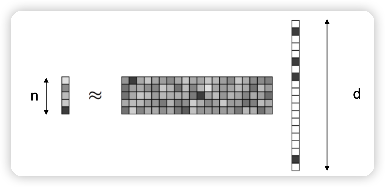
• \(n << d\).

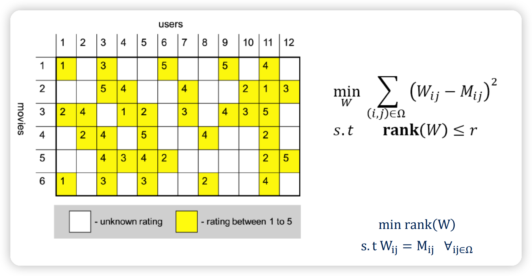
b) Matrix completion

\(\begin{array}{ll} \min _{W} \sum_{(i, j) \in \Omega}\left(W_{i j}-M_{i j}\right)^{2} \\ \text { s.t } \quad \operatorname{rank}(W) \leq r \end{array}\).

• \(\rank (W)\) : non-convex

3. Dyads ( Rank=1 matrix )

(1) Dyad란?

\(\mathrm{A} \in \mathbf{R}^{\mathrm{m}, \mathrm{n}}\) 는 아래와 같이 적을 수 있다면, dyad 라고 한다.

• \(A=p q^{T}\),
  • where \(p \in \mathbf{R}^{\mathrm{m}}, \mathrm{q} \in \mathbf{R}^{\mathrm{n}}\).
• \(A_{i j}=p_{i} q_{j}\),
  • where \(1 \leq i \leq m, 1 \leq j \leq n\).

Dyad의 의미

• (1) \(A\)의 column : \(p\) 칼럼에 \(q\) 만큼의 스케일을 곱한 column
• (2) \(A\)의 row : \(q^T\) 로우에 \(p\)만큼의 스케일을 곱한 row

(2) Sum of dyads ( Rank=r matrix )

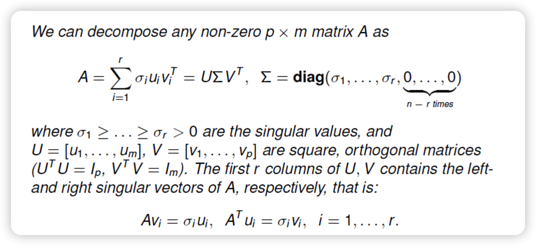
SVD 이론에 따르면, 그 어떠한 matrix도 아래와 같이 sum of dyads로 나타낼 수 있다.

\(\mathrm{A}=\sum_{i=1}^{r} \mathrm{p}_{\mathrm{i}} \mathrm{q}_{\mathrm{i}}^{\mathrm{T}}\).

• for vectors \(\mathrm{p}_{\mathrm{i}}, \mathrm{q}_{\mathrm{i}}\) that are mutually orthogonal.

이렇게 표현하는 이유?

\(\rightarrow\) 행렬을 “보다 간단한(simple) 행렬”들의 합으로 나타낼 수 있으므로!

4. SVD

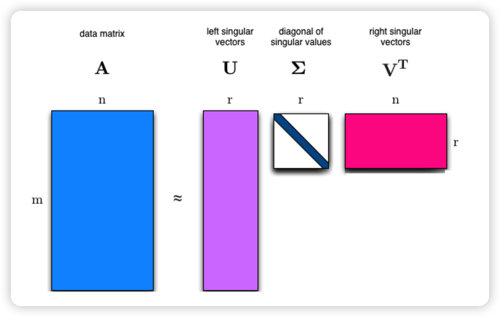
SVD의 해석

• 식 : \(A=\sum_{i=1}^{r} \sigma_{i} u_{i} v_{i}^{T}\).
• sum of dyads로 나타냄을 알 수 있다

기타

• \(u_i\) & \(v_i\) 는 “normalized” & 서로 orthogonal
• \(\sigma_i > 0\) : “strength”of 해당 dyad

5. PCA

(1) PCA란?

Principal component analysis (PCA) is a technique of unsupervised learning,

widely used to “discover” the most important, or informative, directions in a data set,

that is the directions along which the data varies the most.

\(\rightarrow\) 정보를 최대한 보존하는 ( 분산을 최대화하는 ) 축을 찾기!

이름 그대로, PCA를 통해 PC(Principal Component, 주성분)을 찾는다

( = orthogonal directions of maximal variance )

푸는 방법 : covariance matrix의 eigenvalue decomposition

• 기존 data matrix에 대한 factor model로써 해석할 수 있다.

(2) Variance Maximization problem

NON-convex problem이다.

Notation

• \(S\) : covariance matrix
• \(A\) : data matrix
  • \(A_c\) : “centered” data matrix

Variance Maximization problem 푸는 법

• (1) \(S\)의 EVD ( Eigen Value Decomposition )
  • \(\max _{x} x^{T} S x: \mid \mid x \mid \mid_{2}=1\).
  • EVD of \(S\) : \(S=\sum_{i=1}^{p} \lambda_{i} u_{i} u_{i}^{T}\)
    • with \(\lambda_{1} \geq \ldots \lambda_{p}\)
    • \(U=\left[u_{1}, \ldots, u_{p}\right]\) is orthogonal \(\left(U^{T} U=I\right)\)
  • \(\text{argmax}_{x: \mid \mid x \mid \mid_{2}=1} x^{T} S x=u_{1}\).
    • \(u_1\) : eigenvector of \(S\) ( 가장 큰 e.v \(\lambda_1\)에 해당하는 eigenvector )
• (2) \(A_c\)의 SVD ( Singular Value Decomposition )

6. Low Rank Approximation

Notation

• \(A\) 행렬 : \(p\times m\)
• \(k\)-th rank approximation
  • \(k \leq m\) 인 정수

\(k\)-rank approximation problem

• \(A^{(k)}:=\arg \min _{X} \mid \mid x-A \mid \mid_{F}: \operatorname{Rank}(X) \leq k\).
  • where \(\mid \mid\cdot \mid \mid_{F}\) is the Frobenius norm

Solution : \(A^{(k)}=\sum_{i=1}^{k} \sigma_{i} u_{i} v_{i}^{T}\)

• \(A=U \Sigma V^{T}\) : \(A\)에 대한 SVD

Example)

\(A \in \mathbf{R}^{p \times m}\) : time-series 데이터

• 각 row는 하나의 time series이다.
• 즉, \(p\)개의 시계열, \(m\)만큼의 time length
• \(A\) 는 rank one ( 즉 , \(A=u v^{T} \in \mathbf{R}^{p \times m}\) )

위를 정리하자면,

\(A=\left(\begin{array}{c} a_{1}^{T} \\ \vdots \\ a_{m}^{T} \end{array}\right), \quad a_{j}(t)=u(j) v(t), \quad 1 \leq j \leq p, \quad 1 \leq t \leq m\).

해석 1 ( approximation 이전 )

• 각 time series는, \(v\)로 대표되는 (기저) time series의 scaled copy 이다

  ( scaled factor는 \(u\) )

• 우리는 이러한 \(v\)를 일종의 factor로 볼 수 있다.

\(k\)-rank approximation

• \(A=U V^{T}, \quad U \in \mathbf{R}^{p \times k}, \quad V \in \mathbf{R}^{m \times k}, \quad k<<m, p\).
• \(j\)-th row of \(A\) :
  • \(a_{j}(t)=\sum_{i=1}^{k} u_{i}(j) v_{i}(t), \quad 1 \leq j \leq p, \quad 1 \leq t \leq m\).

해석 2 ( approximation 이후 )

• 각 time series는, \(v_1 \cdots v_k\)로 대표되는 \(k\)개의 (기저) time series의 scaled copy 이다

  ( scaled factor는 \(u_1 \cdots u_k\) )

• 우리는 이러한 \(v_i\)들을 일종의 factor로 볼 수 있다.

결론

Factor models

• PCA는 data matrix의 low rank approximation을 가능하게 한다.
  • \(A^{(k)}=\sum_{i=1}^{k} \sigma_{i} u_{i} v_{i}^{T}\).
• \(v_i\) : particular factor
• \(u_i\) : scaling